|
|
|
|
|
|
|
|
Trying a Different Layout Strategy
Adding to the Network Incrementally
CSV Loads Create Interaction Tables
Some Model Properties Cannot be Specified With CSV
Note: This version of the tutorial for Building Networks from Comma-Separated Value Files shows reduced-size screen shots. You can click on any image and see the full-size image in a separate window. To get the version with full-size images, go here.
BioTapestry can construct a complete model hierarchy from a comma-separated value (CSV) file exported by a spreadsheet program. This simple input format also provides an avenue to use BioTapestry as a visualization tool at the end of a computational pipeline, since it is relatively straightforward to create a program that can write out data in the required CSV format.
In this tutorial, you will import a pre-existing CSV file that defines a model hierarchy that matches the one built interactively in the Tutorial on Building Networks from Interaction Tables. So the first step is to download the TutorialSpreadsheetVer2.csv sample CSV file from the BioTapestry web site.
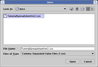
How you save CSV files at a URL depends on your web browser. With Firefox, for example, you would right-click on the above link and select Save Link As... to save the file. After saving TutorialSpreadsheetVer2.csv on your computer, start up a spreadsheet program like Microsoft Excel or OpenOffice Calc and open the file. (Depending on the spreadsheet program, you may need to specify the file type in the file chooser to include .csv files so you can see and select TutorialSpreadsheetVer2.csv.)
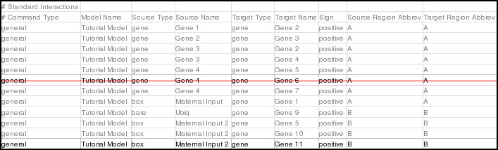
Here is what the file looks like in a spreadsheet program:
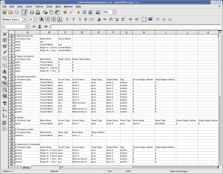
The comments in that file (any row that begins with a cell starting with "#" is treated as a comment) label the required contents of each column, and the file can serve as a template for creating a description of your own network. Remember that if you create a file of this type in your favorite spreadsheet program, you will need to make sure you save it in .csv format so BioTapestry can load it in. BioTapestry cannot read native Microsoft Excel .xls spreadsheet files!
We will now describe the different kinds of instructions you can have in the spreadsheet.
There are three basic types of instructions in the CSV input: model, region, and interaction. Furthermore, the interaction instructions are different for different types of interactions, and there are currently three subtypes for interaction instructions: general, signal, and nodeOnly. The following tables describe the format for each of these instruction types, and we also show where each instruction appears in the tutorial spreadsheet.
In the following table descriptions, bold items are required keywords, items in bold italics need to come from a limited set of possible keywords (which are enumerated), and items in italics should be customized with your own values.
| Column Number | Contents |
|---|---|
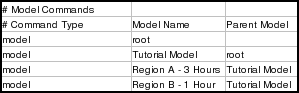
| 1 | model |
| 2 | model name |
| 3 | parent model name |
Notes:
![]() The model hierarchy defined with model instructions must form a tree, i.e.
one and only one model has no parent, all other models have exactly one parent,
and no cycles are permitted.
The model hierarchy defined with model instructions must form a tree, i.e.
one and only one model has no parent, all other models have exactly one parent,
and no cycles are permitted.
![]() Model names must be unique.
Model names must be unique.
![]() Parent model names must reference a model created by another model instruction.
Parent model names must reference a model created by another model instruction.
The following lines in the tutorial spreadsheet are the model instructions:
| Column Number | Contents |
|---|---|
| 1 | region |
| 2 | model name |
| 3 | region name |
| 4 | region abbreviation |
Notes:
![]() The region name and abbreviation must be unique for a given model.
The region name and abbreviation must be unique for a given model.
![]() The top level model cannot have regions.
The top level model cannot have regions.
![]() The model name must match a previously defined model.
The model name must match a previously defined model.
![]() If regions defined for a child model are not specified in the parent model,
they are automatically included in the parent model.
If regions defined for a child model are not specified in the parent model,
they are automatically included in the parent model.
![]() Abbreviations must be no longer than 3 characters.
Abbreviations must be no longer than 3 characters.
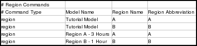
The following lines in the tutorial spreadsheet are the region instructions. If your spreadsheet only defined a single top-level model, it wouldn't contain any of these instructions:
source node type = gene or bare or box or bubble or intercel or slash or diamond
target node type = gene or bare or box or bubble or intercel or slash or diamond
interaction sign = positive or negative or neutral
| Column Number | Contents |
|---|---|
| 1 | general |
| 2 | model name |
| 3 | source node type |
| 4 | source node name |
| 5 | target node type |
| 6 | target node name |
| 7 | interaction sign |
| 8 | source region abbreviation |
| 9 | target region abbreviation |
Notes:
![]() The model name, source region abbreviation, and target region abbreviation must have been defined previously.
The model name, source region abbreviation, and target region abbreviation must have been defined previously.
![]() Interactions defined for the top model do not have source or target regions specified.
Interactions defined for the top model do not have source or target regions specified.
![]() The type for a particular node name must be consistent across all instructions.
The type for a particular node name must be consistent across all instructions.
![]() If an interaction defined for a child model is not specified in the parent model, it is added automatically.
If an interaction defined for a child model is not specified in the parent model, it is added automatically.
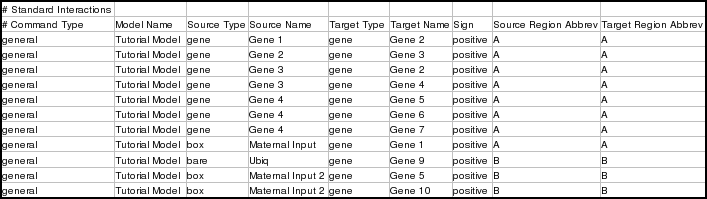
There are two sets of general interaction instructions in the tutorial spreadsheet. The first is for interactions in the Tutorial Model. Note that the spreadsheet does not need to specify any interactions for the top-level model (though it can, if you wish). The top-level model is filled in automatically based upon what is specified for the Tutorial Model:
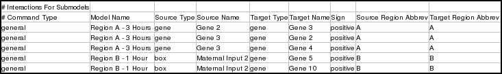
The second set of general interaction instructions is for the two other submodels:
signal type = promoteSig or repressSig or switchSig
| Column Number | Contents |
| 1 | signal |
| 2 | model name |
| 3 | gene |
| 4 | signal source gene name |
| 5 | gene |
| 6 | target gene name |
| 7 | gene |
| 8 | mediated transcription factor name |
| 9 | signal type |
| 10 | source region abbreviation |
| 11 | target region abbreviation |
Notes:
![]() The model name, source region abbreviation, and target region abbreviation must have been defined previously.
The model name, source region abbreviation, and target region abbreviation must have been defined previously.
![]() Interactions defined for the top model do not have source or target regions specified.
Interactions defined for the top model do not have source or target regions specified.
![]() The type for a particular node name must be consistent across all instructions.
The type for a particular node name must be consistent across all instructions.
![]() If an interaction defined for a child model is not specified in the parent model, it is added automatically.
If an interaction defined for a child model is not specified in the parent model, it is added automatically.
There is one signal interaction instruction in the spreadsheet:
node type = gene or bare or box or bubble or intercel or slash or diamond
| Column Number | Contents |
|---|---|
| 1 | nodeOnly |
| 2 | model name |
| 3 | node type |
| 4 | node name |
| 5 | region abbreviation |
Notes:
![]() The model name and region abbreviation must have been defined previously.
The model name and region abbreviation must have been defined previously.
![]() Nodes defined for the top model do not have a region specified.
Nodes defined for the top model do not have a region specified.
![]() The type for the node name must be consistent across all instructions.
The type for the node name must be consistent across all instructions.
![]() If a node defined for a child model is not specified in the parent model, it is added automatically.
If a node defined for a child model is not specified in the parent model, it is added automatically.
There is one standalone node instruction in the spreadsheet:
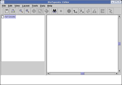
Start with an empty network. Either start up BioTapestry from scratch, or select File->New... from the main menu if you have been previously working on another network:
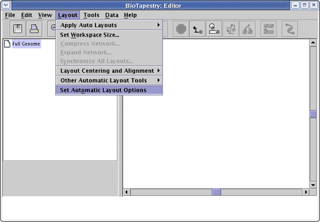
BioTapestry uses its automatic layout algorithms to organize the networks loaded from the CSV file, so we will set some layout options before doing the actual load. From the main menu, select Layout->Set Automatic Layout Options:
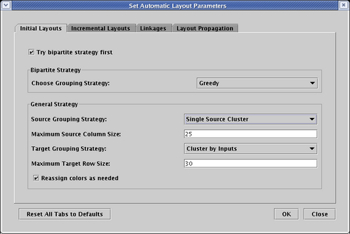
The BioTapestry automatic layout algorithms group source genes (genes with outputs) on the left, and pure target genes (genes with no outputs) on the right. There are a few ways to arrange the hierarchical network of source genes; you can experiment with these options to get the arrangement you prefer. For this network, the Single Source Cluster strategy seems to provide the best result, so on the Initial Layouts tab, set the Source Grouping Strategy to Single Source Cluster. Since there are some genes in the spreadsheet model with both inputs and outputs, the Bipartite Strategy cannot be used on the network, so the setting of the Try bipartite strategy first box won't matter in this case. When the dialog looks like the picture below, click OK:
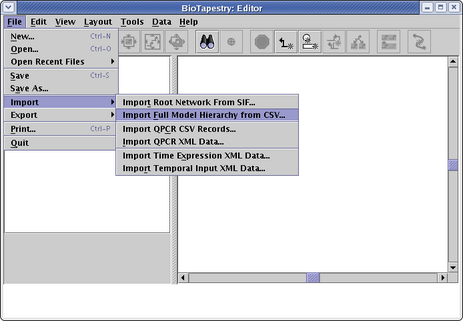
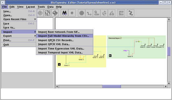
Next, from the main menu, select File->Import->Import Full Model Hierarchy from CSV...:
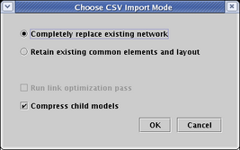
In the dialog box that appears, the two mutually exclusive choices at the top allow you to select how the data in the CSV file will be integrated into the existing network hierarchy. In this case, since we are starting with an empty model, this choice doesn't matter; we can just leave the default selection of Completely replace existing network. However, if you want to build upon an existing network hierarchy and modify it with new data, you would choose Retain existing common elements and layout. That option will compare the existing network hierarchy to the CSV input; both new models and new interactions will be added to the network hierarchy, and missing models and interactions will be deleted. The net effect of this operation is that the new hierarchy will match the one specified in the CSV file, and the existing layout for the network elements retained in the new hierarchy will be kept (as much as possible).
In addition to specifying the basic import strategy, you can also set a couple of other options. If you select the Retain... option, you are given the choice to request a single pass of the link optimizer be run on all the imported networks. This is probably best left unchecked. You are also always provided the opportunity to choose to Compress child models. (Note: on very large networks with very many submodels, this option could cause the program to run out of memory.) You can always leave this unchecked and do a layout synchronization step (with compression) later. For this tutorial, make sure this option is selected. Once you have made your selections as shown below, click OK:
In the file selection box, navigate to the directory where you have placed the TutorialSpreadsheetVer2.csv file, select it, and click Open:
The entire network hierarchy is then constructed, and the Full Genome view appears first:
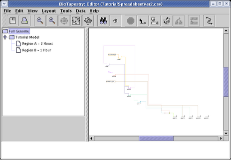
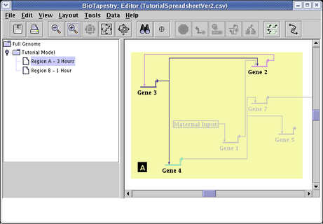
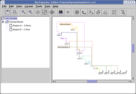
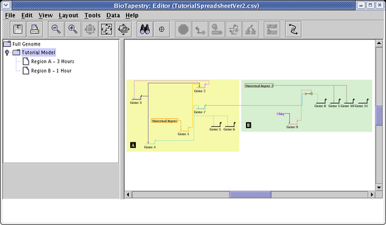
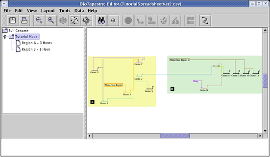
Select the Tutorial Model in the navigation view to see how the automatic layout algorithm arranged the network:
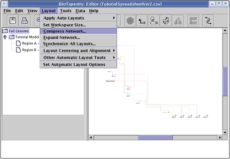
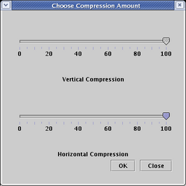
The automatic layout algorithms are designed to handle medium-to-large networks, so here are a few things we can do to improve the layout of this tiny network using some of the automatic layout tools. For example, the top-level Full Genome could be compressed to make it more compact. Go the the Full Genome view, and select Layout->Compress Network...:
Network layout in BioTapestry is based on a fine-grained grid, and full compression (100) will remove all the grid rows or columns in the layout that are devoid of any significant geometric content. (Note that all genes and other nodes are surrounded by some extra padding that will not be deleted even at 100 percent compression.) Set both the Vertical Compression and Horizontal Compression sliders to 100, and click OK:
You can now zoom in much closer while still viewing the entire network, so things are more legible:
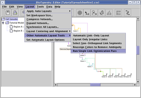
As was mentioned above, the automatic layout algorithms are designed to handle medium-to-large networks, so the link routing patterns that work well for large bundles of links may be overly complex or crowded for a small set of links. For this particular network, doing a link optimization pass can clean things up a bit. From the main menu choose Layout->Other Automatic Layout Tools->Run Single Link Optimization Pass:
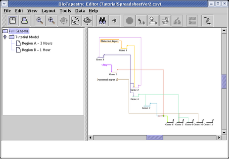
Sometimes you may need to run several passes before things stop changing. You can always toggle the Edit->Undo and Edit->Redo actions to see if you like the changes made by the optimizer. In this case, the optimizations seem to produce a more desirable layout, as shown below. Of course, you can go beyond this and also manually drag nodes around and then use the automatic link layout tools to finish the reorganization. For example, the Layout->Other Automatic Layout Tools->Layout Only Irregular Links tool can reorganize all irregular links after you drag nodes around, or you can right-click on any link segment and select Auto Layout Links Through This Segment to just repair a portion of a link tree.
Some changes you might want to make manually are cosmetic, e.g. moving the Maternal Input 2 box down to remove the link bend. Other desirable changes could improve the presentation of the underlying biology of the network. For example, since the layout algorithm doesn't have access to the time of first expression, it arbitrarily determines the ordering of the feedback loop between Gene 3 and Gene 2. Since Gene 2 expresses first, it may be desirable to change that ordering in the network.
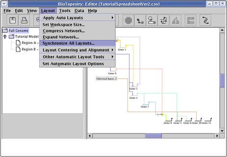
Remember, the Full Genome layout is independent of the layouts in the submodels, to the changes we just made have not been propagated to the submodels. Of course, the compression step we did at this level doesn't make a difference, since the submodel layouts were all originally compressed. But we would like to have the optimized link layouts installed in the submodels. So, from the main menu choose Layout->Synchronize All Layouts...:
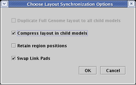
Since there is a duplicate node (Gene 5) in both regions, it is not possible to use a direct copy of the Full Genome layout in the submodel, so the first option is not available. Make sure to select Compress layout in child models and Swap Link Pads. Since trying to retain region positions can sometimes adversely affect inter-region links trees, we typically leave that unchecked. When the dialog matches what is shown below, click OK:
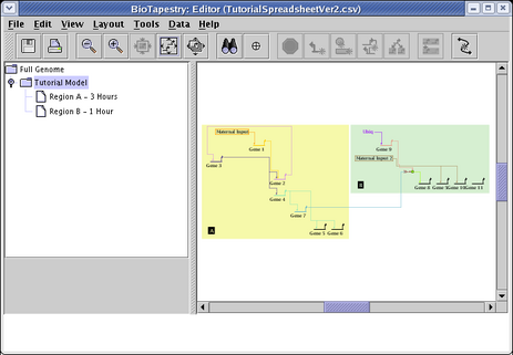
The Tutorial Model should now look like this. Again, you can manually move nodes around and use the automatic link cleanup tools to tweak this to the best possible final arrangement:

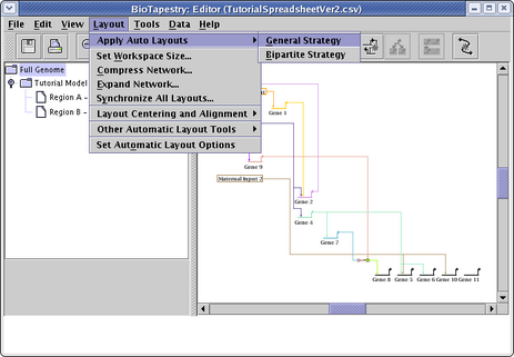
Before loading in the CSV file, we modified the layout options to set the Source Grouping Strategy to Single Source Cluster. We can always go back and try a different layout strategy. To do this, first select the Full Genome model in the navigation panel. Then, from the main menu choose Layout->Apply Auto Layouts->General Strategy:
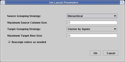
The dialog that appears is set to the defaults we specified back at the beginning of the tutorial. This time, change the Source Grouping Strategy to Hierarchical, and click OK:
If you run through the entire network compression, link optimization, and layout synchronization steps we performed before, and then choose the Tutorial Model, you will see how this other strategy organized the network:
It was mentioned above that a CSV file could be loaded so that existing layouts would be retained (as much as possible). Note that this loading requires that all the retained network elements must be present in the new CSV file; this approach does not treat the incoming CSV file as just a listing of the new elements to be added, but as the definitive complete listing of what is in the new hierarchy.
The new CSV file can add or drop models, regions, or interactions. In this example, we will just add an interaction and drop an interaction. Specifically, for the model Tutorial Model, drop the interaction from Gene 4 to Gene 6 in region A, and add a positive interaction from the box node Maternal Input 2 to Gene 11 in region B. These changes are shown below:
You should also drop the single Gene 11 nodeOnly command, since it is now superfluous:
Instead of editing the spreadsheet directly, you can just load in the TutorialSpreadsheetVer2Pass2.csv CSV file downloaded from the BioTapestry web site.
Again, save the file at the above link, using the method supported by your web browser, e.g. right-click on the above link and select Save Link As.... Then, from the main menu, select File->Import->Import Full Model Hierarchy from CSV...:
This time, in the Choose CSV Import Mode dialog box, choose Retain existing common elements and layout. Do not run a link optimization pass, and again check the Compress child models box. Click OK:

Now go to the Tutorial Model. Note how the layout was retained, with a new link added to Gene 11, and with Gene 6 deleted:
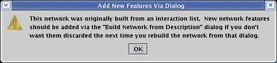
When you import a CSV file to create a network hierarchy, BioTapestry creates a set of underlying interaction tables which are used to generate the networks. The Tutorial on Building Networks from Interaction Tables describes how to work with these tables. These tables then form the definitive definition of the network models. Thus, if you try to make changes to the CSV-loaded network models (this does not apply to layout changes) using drawing or propagation techniques, you will see the following warning message:
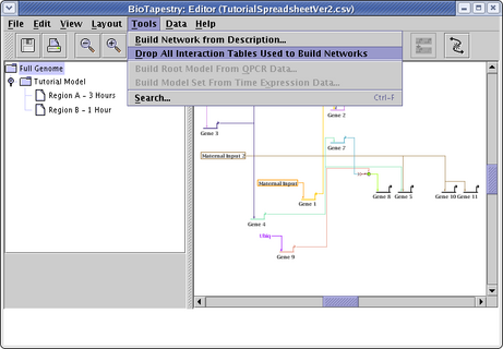
If you wish to just work with the models via interactive drawing techniques following a CSV load, you can choose to drop the interaction table definitions. Just go to the main menu and select Tools->Drop All Interaction Tables Used to Build Networks:
Since CSV loads use interaction tables to build the networks, the limitations of that method apply to CSV loads as well. In particular, activity levels of nodes cannot be specified via CSV imports. As was discussed here in the Tutorial on Building Networks from Interaction Tables, if we want to show Gene 4 (shown below) as inactive in the Region A - 3 Hours submodel, that change must be made by setting the model properties after the CSV load. The problem is that these changes disappear following the next CSV load, if you are adding to the network incrementally. This is a critical shortcoming, which needs to be addressed in a future version of BioTapestry. In the meantime, be aware that modifications like this need to be redone if you do incremental CSV imports.