|
|
|
|
|
|
|
|
Building Experimental Data Tables
Entering Time Course Data Manually
Entering Time Course Data from a File
Entering Temporal Input Data Manually
Entering Temporal Input Data from a File
Creating Hourly Dynamic Models
Setting up Custom Associations to Data
Note: This version of the BioTapestry Dynamic Submodels Tutorial shows reduced-size screen shots. You can click on any image and see the full-size image in a separate window. To get the version with full-size images, go here.
In the introductory Quick Start Tutorial, you learned how to draw a top-level model and then derive a multi-level model hierarchy from it. In that example, all of the models in the hierarchy were static, i.e. you manually specified every element to include in those networks, and each model showed a static snapshot of the network.
In this tutorial, we will cover how to create dynamic submodels, where data tables are used to automatically determine the active network elements, and user can use a time slider to see a dynamic presentation of the network behavior:
Dynamic submodels are driven by tables of experimental data that indicate the temporal and spatial expression of the network elements, as well as when the inputs into each are active. So the first part of this tutorial will discuss how to build these tables and populate them with data. The second part will then discuss how to build the dynamic submodels that access these tables.
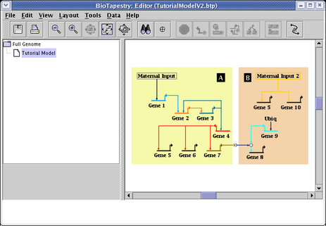
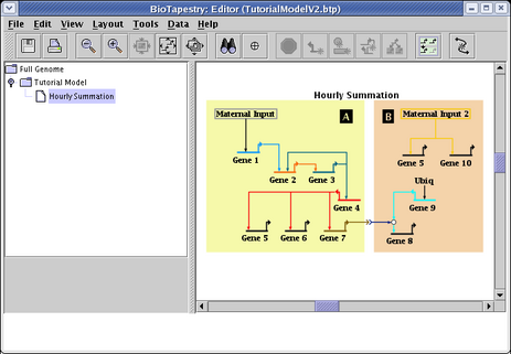
Although the data tables determine what network elements are shown as active in the dynamic submodels, you still need to first construct the top-level model and the top-level submodels manually. There are various ways to do this, but that topic is covered in other tutorials. To learn one way to build these models, begin with the Quick Start Tutorial. The model we start with in this tutorial is shown below. While you can create it yourself if you wish (and if you do, give the intercellular node the name Signal, and the bubble node the name Interaction), the easiest way to get started is to download and save the file TutorialModelV2.btp.
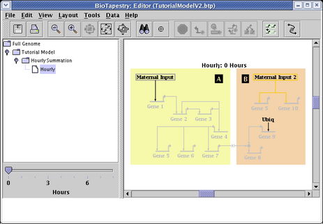
How you save the file in the previous link depends on your web browser. With Firefox, for example, you would right-click on the above link and select Save Link As... to save the file. After saving TutorialModelV2.btp on your computer, start the BioTapestry Editor and open the file. You should see this:
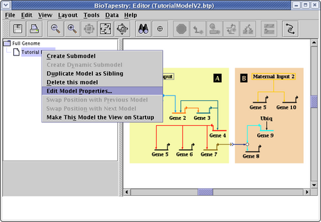
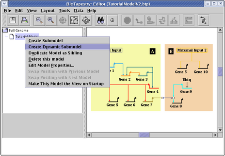
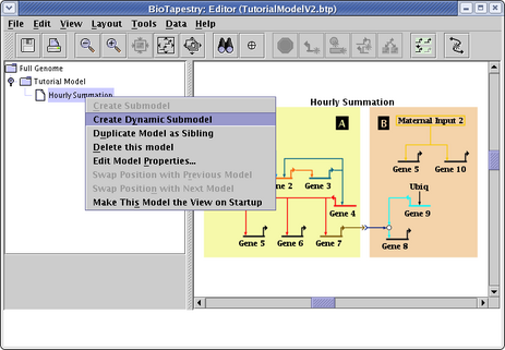
Since we are going to create dynamic submodels, we need to start by assigning time bounds to the parent submodel. So right-click the model Tutorial Model in the navigation view and select Edit Model Properties... from the menu:
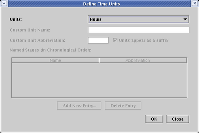
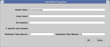
In the Edit Model Properties dialog, check the box labeled Specify time bounds. If you have created this model yourself, checking this box may cause the Define Time Units dialog to appear immediately, since you need to specify what time units you will be using for the model. If it appears, set Units to Hours and click OK:
The TutorialModelV2.btp already has the units defined, so after checking the box, just fill in the times as 0 and 8 hours, and click OK:
Dynamic models are driven by two sets of data tables. The time course data tables indicate the regions and times that a gene (or other network node) is expressing, while the temporal input data tables specify the regions and times that the inputs to a gene (or other network node) are active. There are two ways to populate these tables: you can either enter the data manually using interactive editing dialogs, or import the data from XML data files created elsewhere. This tutorial will cover both methods for each type of table, starting first with how to enter the data manually.
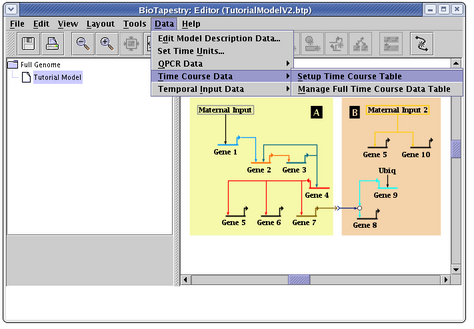
The first step in building the data tables is to lay out the time course data table, by specifying what regions and times are included in it. From the main window menu, select Data->Time Course Data->Setup Time Course Table:
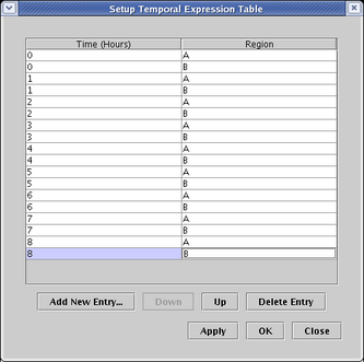
In the resulting dialog box, click on the Add New Entry... button and enter the values 0 for Time and A for Region. Continue to do this until you have alternating entries for regions A and B for 0 to 8 hours, then click OK:
Then, enter in the experimental data for each node in the network. For Gene 1, right-click on the gene (Note to Mac users: if you're using a one-button mouse, press the Control key while clicking the mouse to do this) and select Manage Time Course Data->Edit Data... from the menu:
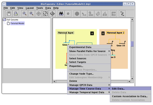
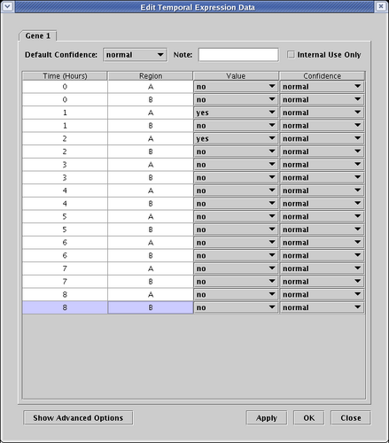
This brings up the dialog that allows you to edit the data table for Gene 1. Since Gene 1 is expressing at 1 and 2 hours in Region A, and is off otherwise, select the entries in the Value column of the table accordingly, and click OK (to save time, you can leave entries at noData for now instead of setting them to no if you wish; the visual effect in the hourly views is the same, though the annotation in the experimental data displays will be wrong):
Entering in data for all the remaining genes nodes works exactly the same way. Note that you will only need to click on one copy of Gene 5 in one region to enter data globally for all regions. If you wish to manually add all the time course data for the network, you can now fill in all the data according to the following table. However, it is faster and easier to complete the job by importing the data from an existing file, as described in the next section.
| Name | Region A | Region B |
|---|---|---|
| Maternal Input | 0 - 2 hr | None |
| Maternal Input 2 | None | 0 - 1 hr |
| Gene 1 | 1 - 2 hr | None |
| Gene 2 | 2 - 8 hr | None |
| Gene 3 | 3 - 8 hr | None |
| Gene 4 | 4 - 8 hr | None |
| Gene 5 | 5 - 8 hr | 1 - 2 hr |
| Gene 6 | 5 - 8 hr | None |
| Gene 7 | 5 - 8 hr | None |
| Signal | 5 - 8 hr | None |
| Gene 8 | None | 7 - 8 hr |
| Gene 9 | None | 1 - 8 hr |
| Gene 10 | None | 1 - 2 hr |
| Ubiq | None | 0 - 8 hr |
| Interaction | None | 6 - 8 hr |
The time course data file for this tutorial is available from the BioTapestry web site: TutorialExpressionDataV2.xml. Save the file to your computer (e.g. for Firefox, right-click on the link and do a Save Link As... in your browser):
This file, as well as the file for temporal input data discussed below, are human-readable XML text files. You should look at these files in a text editor to understand how they are organized, and use them as the template for building your own data input files for your own models.
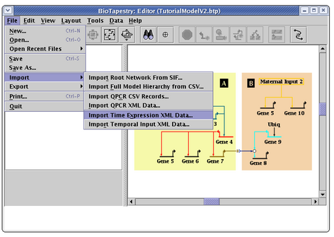
To load the saved expression data file into BioTapestry, go to the main menu and select File->Import->Import Time Expression XML Data...:
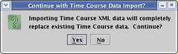
A dialog box will pop up to warn you that existing data will be lost (an import does not append to existing data, but replaces it). Click Yes:
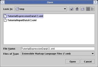
In the file chooser dialog that pops up, set Files of Type to Extensible Markup Language Files (*.xml), select TutorialExpressionDataV2.xml, and click Open:
All the time course data has now been loaded, and BioTapestry now has enough information to show when and where each gene is active during the eight hour display period. Next, you need to provide data on when each input is active for each gene.
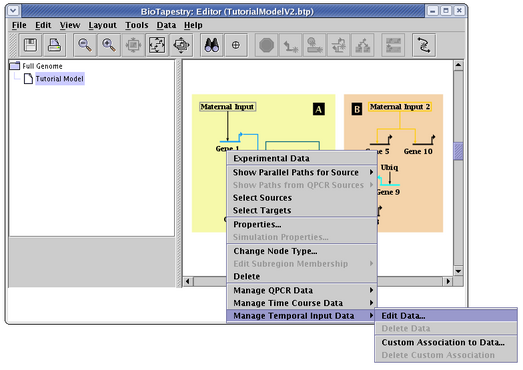
Again, you will see how the temporal input data is organized by manually entering some values, and then shortcut the process by importing the data from a file. Unlike the time course data tables, the temporal input data tables do not require a preliminary setup step, so you can immediately begin adding temporal input data for the model by right-clicking on Gene 1 and selecting Manage Temporal Input Data->Edit Data... from the menu:
This brings up the dialog to enter the Gene 1 data. Click on Add New Entry... and type in Maternal Input for Input, A for Region, and 2 for Maximum Time. Then click OK:
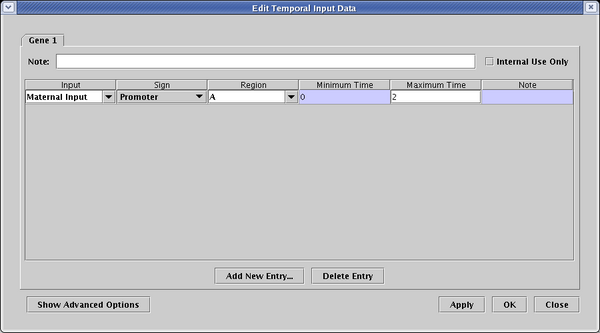
(Once you start building up the tables with data, the input and region values can frequently be selected from drop down values instead of having to be typed in.)
You can then proceed on to fill in the data table for all the other nodes. It is easier to load the data from a file, as described in the next section, but if you wish to manually add all the remaining data for the network, use the values in the table below for each node (except for Maternal Input, Maternal Input 2, and Ubiq, which have no inputs). Note that Gene 2, Gene 5, and the Interaction bubble both have two inputs, and thus each will have two rows in its table. All these interactions have a Sign of Promoter:
| Name | Input | Region | Times |
|---|---|---|---|
| Gene 1 | Maternal Input | A | 0 - 2 hr |
| Gene 2 | Gene 1Gene 3 | AA | 1 - 2 hr 3 - 8 hr |
| Gene 3 | Gene 2 | A | 3 - 8 hr |
| Gene 4 | Gene 3 | A | 3 - 8 hr |
| Gene 5 | Gene 4Maternal Input 2 | AB | 4 - 8 hr 0 - 2 hr |
| Gene 6 | Gene 4 | A | 4 - 8 hr |
| Gene 7 | Gene 4 | A | 4 - 8 hr |
| Signal | Gene 7 | A | 5 - 8 hr |
| Gene 8 | Interaction | B | 6 - 8 hr |
| Gene 7 | Gene 4 | A | 4 - 8 hr |
| Interaction | Gene 9Signal | BB | 1 - 8 hr 6 - 8 hr |
| Gene 9 | Ubiq | B | 0 - 8 hr |
| Gene 10 | Maternal Input 2 | B | 0 - 2 hr |
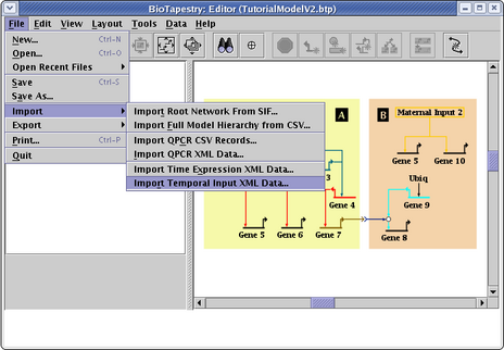
The input file is available at TutorialInputDataV2.xml. Save it to your computer just like the previous data file, then load the data file into BioTapestry by going to the main menu and selecting File->Import->Import Temporal Input XML Data...:
The steps to go through for loading this file match those for the time course data; you acknowledge a warning about overwriting existing data, be sure to set Files of Type to Extensible Markup Language Files (*.xml) so you can see the XML files in the file chooser, and select the TutorialInputDataV2.xml file. Once this is loaded, the program has all the information it needs to drive the dynamic models.
In this tutorial, you will create two levels of dynamic submodels. The first one will be a summation model, which will show all the active genes and interactions that occur over a span of time, "integrating" all the relevant time points into a single display. This can be very useful to get an overview of activity. The second model, an hourly model, will be created as a submodel of the summation model, and will show the activity on an hour-by-hour basis.
To begin, right-click on the Tutorial Model entry in the navigation tree, and select Create Dynamic Submodel in the menu:
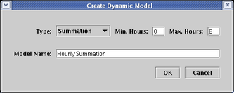
In the dialog box, leave Type at Summation. Since the parent model has already been defined to have a time span from 0 to 8 hours, you also should not have to change the time settings. Just specify the Model Name to be Hourly Summation and click OK:
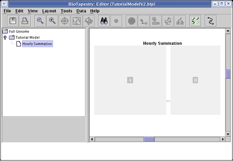
Select the new Hourly Summation submodel in the navigation tree, and you will see regions A and B grayed out:
In complex networks, you may want to create several summation models at the same level in the collection of models, with each separate model only including one or two of all the possible regions. However, in this simple network, include both regions in this single model. A region is included by first clicking on the Choose Subset of Parent button in the toolbar:
The cursor then changes to a crosshair, and the program will now stay in this choosing mode until you press the Esc key, or click on the Cancel Current Add (the stop sign) or Choose Subset of Parent button. Move the crosshair cursor over the grayed-out region A and click the mouse, and A will then be part of the submodel:
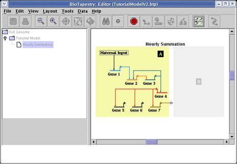
Continuing in choose mode, select region B, and then exit choose mode. The Hourly Summation submodel is now complete. BioTapestry is using the underlying data tables to determine which network elements are included, and since all network elements are active at least some time during the 8 hour period, they are all included. Thus, this model should look exactly like the parent model in this particular situation (except for the title). If you had set the time range for this model to be a smaller interval, it would have included only a subset of the parent network:
Finally, create the last model by right-clicking on the Hourly Summation model in the navigation view and selecting Create Dynamic Submodel:
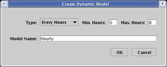
This time, choose Every Hours for Type, and set the Model Name to Hourly. By default, the mimimum and maximum times are set to the parent model values; keep these settings in this example. Click OK:
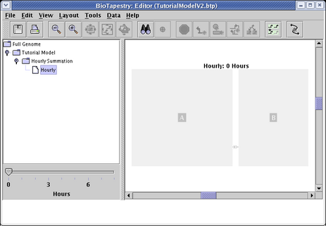
Just as with the previous dynamic model, when you now go to select the Hourly model, it appears empty:
You use the same procedure as before: click on the Choose Subset of Parent button in the toolbar, click on regions A and B with the cross-hair cursor, then exit the selection mode:
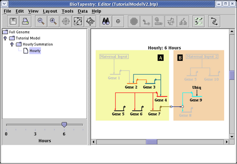
With this new hourly model, you can now slide the hour selection slider, and can see how the state of the network changes over eight hours on an hour-by-hour basis:
In the TutorialModelV2.btp model we have been using in this tutorial, each node in the top-level model has a unique name. Even the signal node and bubble node, which appear to be nameless, have unique names (Signal and Interaction), and the presentation properties for those nodes are set to hide those names. In fact, if you are setting up dynamic models, this is the preferable approach for creating a "nameless" node, instead of creating the node with an empty name (which is legal for all non-gene nodes) and then setting up a custom association, as we detail in this section.
Genes are always required to have a unique, non-empty name, but other nodes can have the same name, including no name. This can be useful. For example, you may want to show a different Ubiq input into a variety of different genes, where each of these Ubiq nodes turns on and off at different times. This would mean that each node would need to be driven by different underlying data tables. Thus, a Ubiq input into Delta would be driven by a table labeled DeltaUbiq, while a distinct but identically named Ubiq input into Hnf 6 would be driven by a table labeled Hnf6Ubiq.
This flexibility is provided through custom associations to data. As long as you tag the underlying time course and temporal input tables with a name that is identical to the displayed node in the network (the match is case-insensitive), the software associates the tables with the node automatically. But if a data table has a different name from the node, you need to explicitly tie the two together.
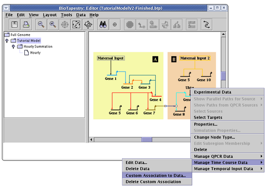
To set up a custom association for time course data, right-click on a node and choose Manage Time Course Data->Custom Association to Data. In the example below, we are going to set an association for the Ubiq input into Gene 9:
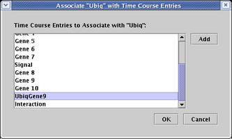
This pops up a dialog, where you can select the name(s) of the time course tables to associate with the node. By Ctrl-clicking on multiple entries, you can tie the node to multiple underlying tables, and you can click on the Add button to add new entries to the list. The following example demonstrates what you would need to do if the XML file you loaded had named the Ubiq entry as UbiqGene9 instead (which it didn't); you would select it from the list and click OK. Assuming that you have been following along with the tutorial, you are probably actually seeing that Ubiq is selected, and you don't need to do anything: just click Cancel.
In a similar fashion, you can set up custom associations for the temporal input data and QPCR data. Furthermore, regions (such as the regions A and B in this tutorial) can have custom region associations set up if the name of the region in the network is not identical to the region references in the data tables. To do this, you would right-click on an empty part of the colored region rectangle to bring up the menu for the region, and proceed in a similar fashion.