|
|
|
|
|
|
|
|
This "Quick Start" tutorial is designed to walk you through the basic steps involved in building a multi-level genetic regulatory network (GRN) model hierarchy in BioTapestry by drawing the network elements. While there are other ways to create models (e.g. using lists of interactions entered using dialog boxes, creating dynamic models based on experimental data tables, etc.), the approach used in this tutorial is very useful and is the easiest to learn.
The topics being covered here are:
Understanding the BioTapestry Model Hierarchy
Populating the Lowest-Level Submodels
Further Study and Other Resources
Note: This is the version of the Quick Start Tutorial with full-size screen shots. To get the version with reduced-size images, go here.
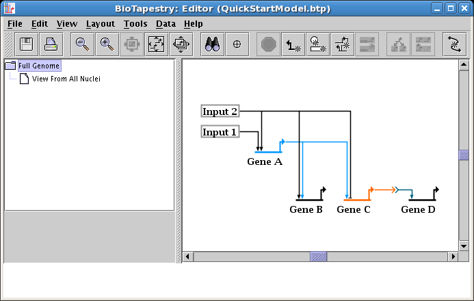
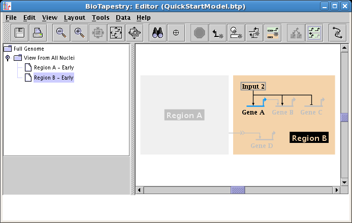
To use BioTapestry effectively, it is essential to understand how it represents a genetic regulatory network (GRN) as a hierarchy of models. The same underlying GRN behaves differently in different cell types, spatial domains, environmental conditions, and at different times. BioTapestry is designed to help the user to organize these varying views of the network state in a coherent fashion, and it does this by using a multi-level model hierarchy. For example, the following figure shows how the Tutorial Model you will be building uses the model hierarchy to illustrate different aspects of a GRN. Note how the model hierarchy is navigated by selecting different models in the tree view on the left side:
Starting from the upper left, and going clockwise, the three views above are as follows:
![]() The top-level model, named Full Genome, provides a summary of all
inputs into each gene, regardless of when and where those inputs are relevant. One and only one copy of each network element is shown.
The software enforces the requirement that all network elements that appear in lower-level models must be present in this model.
The top-level model, named Full Genome, provides a summary of all
inputs into each gene, regardless of when and where those inputs are relevant. One and only one copy of each network element is shown.
The software enforces the requirement that all network elements that appear in lower-level models must be present in this model.
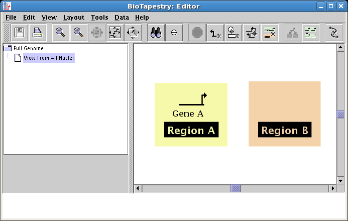
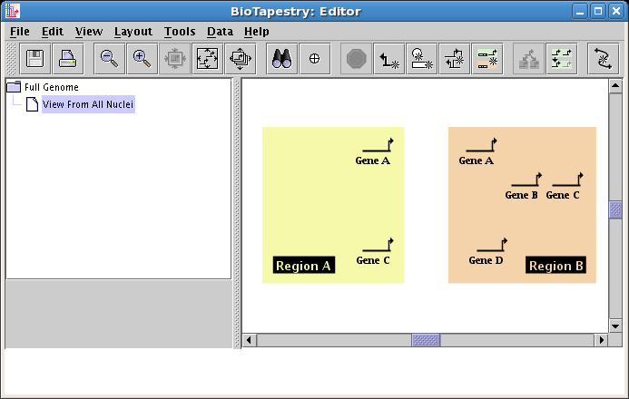
![]() The next model down, named View From All Nuclei, is derived from the
top-level model, and introduces the concept of regions. Each region in this model contains a subset of the top-level network. This
presentation allows us to show how the common underlying network behaves differently in different regions. In this particular example,
this model is showing the relevant network elements active in each region over the entire time period of interest.
The next model down, named View From All Nuclei, is derived from the
top-level model, and introduces the concept of regions. Each region in this model contains a subset of the top-level network. This
presentation allows us to show how the common underlying network behaves differently in different regions. In this particular example,
this model is showing the relevant network elements active in each region over the entire time period of interest.
![]() The lowest level models, e.g. the model named Region B - Early, describes
a specific state of the network at a particular time and place. Inactive portions of the network are indicated in
gray, while the active elements are shown colored.
The lowest level models, e.g. the model named Region B - Early, describes
a specific state of the network at a particular time and place. Inactive portions of the network are indicated in
gray, while the active elements are shown colored.
Note how each of these models provides a different perspective on the GRN. By looking at the top-level model, you can see each gene's full regulatory program within a GRN. However, to see effects which are highly dependent on specific temporal and spatial conditions, such as functional blocks in the network (e.g. mutual exclusion), the lowest-level models are appropriate.
BioTapestry is centered on this hierarchical approach, and it's important to keep this in mind when creating a model, since the model hierarchy imposes certain restrictions on how models can be organized. For example, a gene or link cannot be added to a lower level model unless it also present in the models above it in the hierarchy. The flip side of this rule is that deleting a network element from a model automatically removes it from all the models below it. Another requirement is that regions do not exist in the top-level model, and multiple copies of genes cannot be drawn in the top-level model. In this tutorial, you will see how to work within this framework when using BioTapestry.
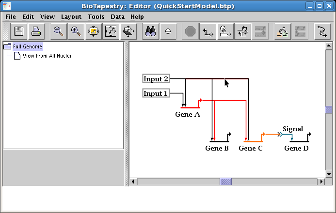
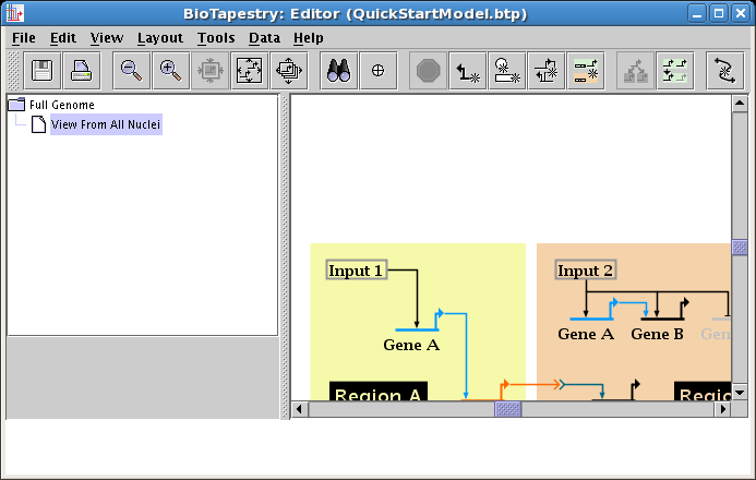
We will be building the model shown below in this tutorial. The model consists of two regions, where there is signaling from Region A to Region B. Note that some network elements are common to both regions, while some are unique. In addition to the network view shown here (the View From All Nuclei), this model hierarchy also consists of a top-level network, as well as two submodels that depict the network state in each of the regions at an early time point. This hierarchy is depicted in the navigation panel on the left:
While this tutorial is designed to step you through the process of building this model, you can also download the completed Quick Start tutorial model from here, (right-click the link and choose to save the file on your computer).
BioTapestry is a web-based application run using Java Web Start, so it should run on most computers (e.g. Windows, Mac, and Linux). To run it, go to the BioTapestry.org web page and click on the link that says "Click HERE" (see below). Java Web Start downloads the software to your computer and caches a local copy, but since it allows you to create a desktop shortcut to start up BioTapestry without having to visit the web page, and since it allows you to run the application without being connected to the Internet, it operates much like a locally installed program. However, the Java Web Start system will insure that your version of the software is kept up-to-date as new versions are released, since it will check back with the BioTapestry.org server to see if updates are available.
One thing to keep in mind is that although the application is maintained by the Java Web Start system, your work files are saved on your local computer, not on the BioTapestry.org server.
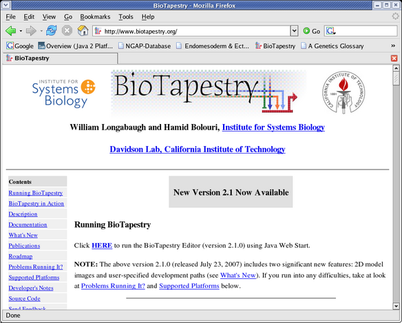
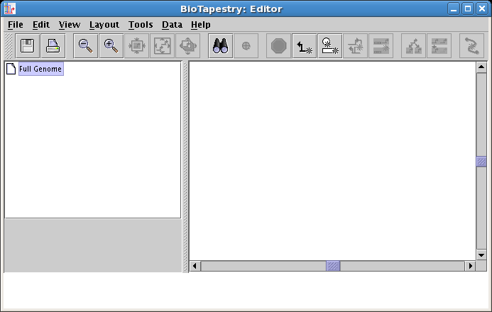
After clicking on the link, if you have not run the program on this computer before, you will need to accept security certificates that insure the software you are running is guaranteed to originate from the Institute for Systems Biology and Sun Microsystems. Then you will see the BioTapestry Editor appear with an empty model:
Up until the release of Version 3, the creation of a model hierarchy would require you to always draw your network in the top-level model first, and then use this network as the basis for creating all the models below it in the hierarchy. That method is still fully supported, but starting with Version 3, you can begin to draw your network at any level in the model hierarchy. If you begin by drawing a model lower down in the hierarchy, BioTapestry automatically adds the necessary network elements to models above it to maintain the required consistency between the models. If your intended final product is a model containing regions, it is probably easiest to begin your work with the second-level model.
For this tutorial, you will begin by drawing the second-level View From All Nuclei model. As you draw genes, nodes, and links, the program will automatically add these elements into the top-level Full Genome model. After you have finished this model, you will spruce up the layout in the top-level model, as that model has a network layout that is independent of the layouts in the models below it, and it pretty quickly gets out of sync with those layouts as you move things around. While there is a tool to help keep the top-level model layout in sync (see Layout->Propagate Layout to Full Genome Model...), we will use a manual layout cleanup process to cover several very important layout editing operations in this tutorial.
After you have finished the layout cleanup, you will complete the tutorial by creating and populating two submodels at the bottom of the model hierarchy.
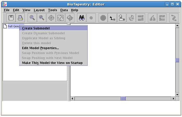
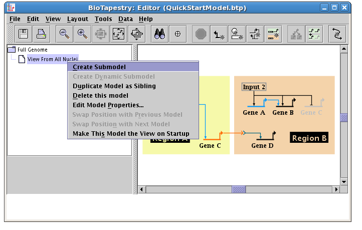
To begin, create the View From All Nuclei model. Do this by right-clicking on the Full Genome entry in the navigation pane on the left side of the BioTapestry window. (Note to Mac users: if you're using a one-button mouse, press the Control key while clicking the mouse to do this.) In the pop-up menu that appears, select the Create Submodel entry:
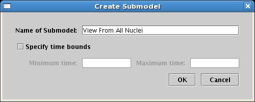
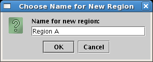
In the dialog box that pops up, type the name of the model, View From All Nuclei, into the Name of Submodel field, and click OK:
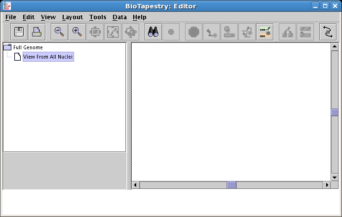
This creates the new model, and you will see it in the navigation pane, but note that it has not yet been selected! Click on the new model entry to select it, and you will now be looking at the empty model you will be drawing into:
Recall from the discussion above that models below the top level contain regions. In fact, these models are required to have at least one region. Genes and nodes can only be drawn inside a region, so you will note that the tool bar has inactive buttons for drawing anything but new regions, as shown below. NOTE: If you are not seeing this (i.e. the Add Region... button is inactive, but the Add Gene... and Add Other Node... buttons are active), you need to make sure you have selected and are viewing the View From All Nuclei model:

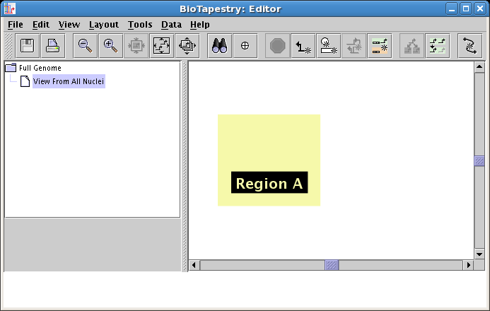
Click on the Add Region... button, and in the dialog box that appears, set the region name to Region A, and click OK:
Now as you move the mouse over the network workspace pane, you will see a colored square named Region A move with it. Locate the square on the left side of the pane, as shown below, and click to place it:
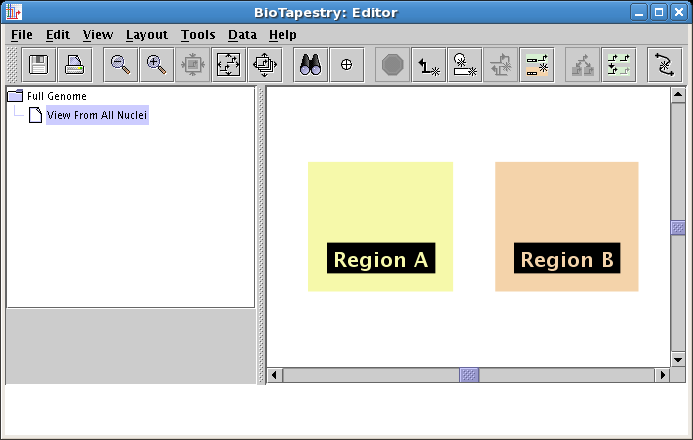
Follow this same set of steps again, except name the region Region B, and place it on the right side, as shown below:
Now that the regions have been created, you will draw the genes and nodes.
You will draw all the genes first. Start by clicking on the Add Gene... button:

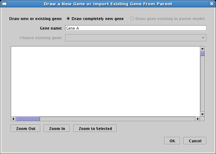
This brings up a dialog, shown below. Since this will be the first gene created, and the top-level model is empty, you are restricted to the Draw completely new gene option. However, as you will see shortly, when genes are present in the top-level model, you are also given the option of selecting one of those genes to draw. For now, name the new gene Gene A and click OK:
A "floating gene" appears, following your mouse cursor. Locate it inside Region A where you want to place it and click the mouse. If you want to cancel the placement, just click on the Stop Sign button on the toolbar or press the Esc key on the keyboard. Also, if you make a mistake, you can always use the Edit->Undo feature on the main menu. Once you have placed the gene, your model should look like this:
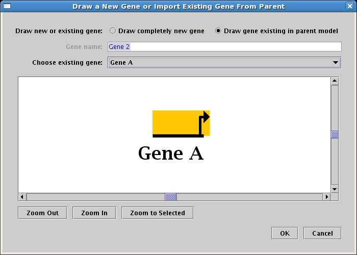
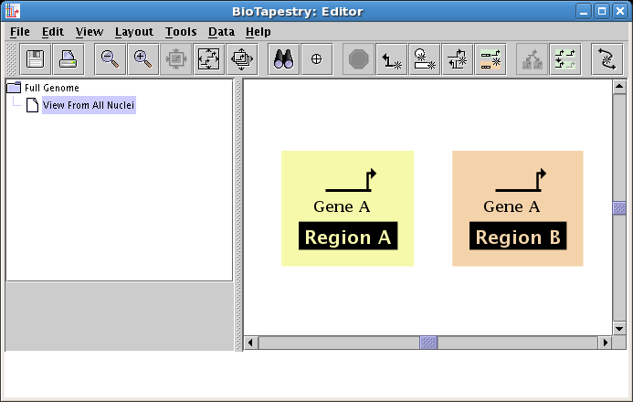
Gene A is also present in Region B, so you will add it now. Again, click on the Add Gene... button and the same dialog appears (see below). However, when you first drew Gene A, it was automatically added to the top-level model. (Remember that the top-level model is required to have one and only one copy of every gene present in the models beneath it in the hierarchy.) So since we are adding another copy of Gene A, choose the Draw gene existing in parent model option at the top, and select Gene A in the Choose existing gene drop-down box. When you do this, the large model view panel will show Gene A selected, as it appears in the top-level model. Note that the model view panel is just a display of what is chosen in the drop-down box; you cannot click on it to select items.
One thing to note is that if you instead chose the Draw completely new gene option and named it Gene A, the system will let you continue, but it would first pop up a dialog box to let you know that you are actually going to be placing a gene that already exists in the top-level model, not creating a completely new one. There can be no two genes in the Full Genome model with the same name (case and spaces are ignored when making this check).
Although there can be only one Gene A in the top-level model, you are about to have two Gene As in the model you are creating. However, the second copy will exist in Region B, since below the top-level model, each region can have a complete copy of the top-level model in it. Once this second Gene A is added, you will not be able to add any more copies of Gene A, since you only have two regions, and it is not possible to add a gene that is not in a region.
Now continue by clicking on the OK button:
Again, a "floating gene" appears and tracks your mouse cursor. Locate it in Region B, and click to place it:
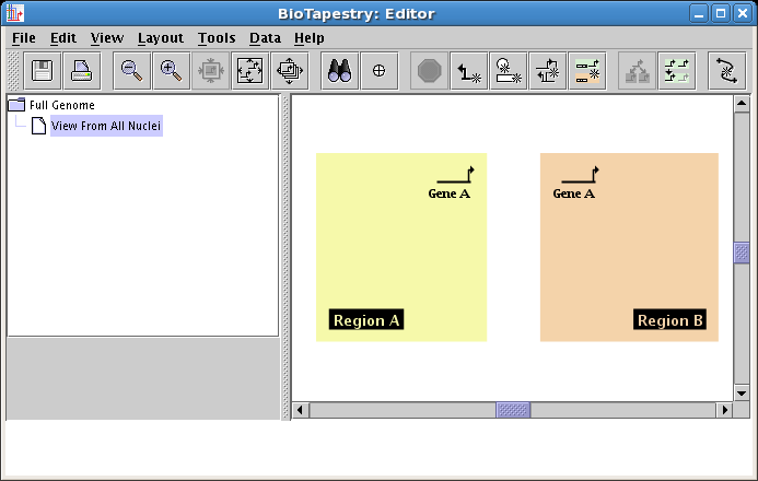
To keep adding genes, we are going to have to make the regions bigger. The region boxes automatically resize to contain the nodes and genes inside them, as well as the region name block. So to make them bigger, we will just drag the region labels. But first, we want to zoom out to get a wider view of the workspace. The various zoom buttons on the toolbar, shown below, are used for this. From left to right, there are buttons for: zooming out a step, zooming in a step, zooming to show selected items (you need to have selected something to activate this), zooming to bound the current model, and zooming to bound all the models in the hierarchy:

Click the Zoom Out button a couple of times, then use the mouse to drag the two region labels down and away from the center to create more room:
Now add the rest of the genes, placing one copy of Gene B in Region B, a copy of Gene C in each region, and a copy of Gene D in Region B. Note that your second copy of Gene C will be best created by again specifying Draw gene existing in parent model in the dialog. Your model should now look like this:
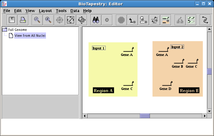
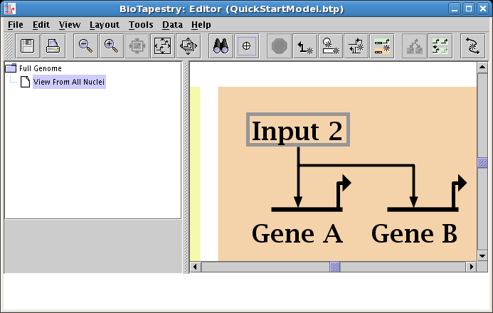
Next, you need to add two boxes named Input 1 and Input 2, which will represent, e.g., anisotropically distributed maternal inputs in the embryo. These non-gene nodes are added by clicking on the Add Other Node... button:

This brings up the dialog shown below, which is very much like the dialog for adding genes, except there is the additional choice for Node type. Select Box for the type, name the node Input 1, and click OK to place the node in the same fashion as placing genes:
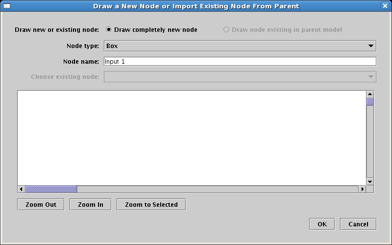
Place the Input 1 box node in Region A, then repeat these steps, instead placing a box node named Input 2 into Region B. Your model should look like this:
It is important to note that there is no requirement for distinct non-gene nodes to have unique names in the top-level model, though they cannot have the same name as a gene. One consequence of this is that when you have multiple nodes with the same name, it is important to keep track of which node in the top-level model you are specifying when you choose to draw it in a child model. While it might not seem to make a difference if there are no links between nodes, it is crucial once you have the nodes linked together in a network. This is where the network view in the dialog box can be invaluable!
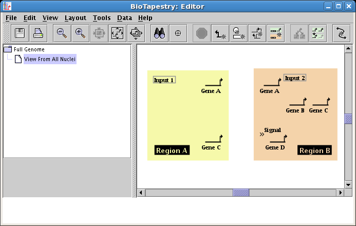
The final node to draw will be a signal node, located in Region B. To do this, you will need to select a Node type of Intercellular in the dialog, and name the node Signal. Place the signal node as shown:
You want to make a habit of saving your work. So now choose File->Save As... and save the model (we are calling it QuickStartModel.btp):
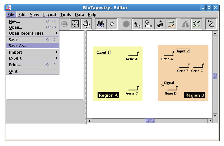
Note that the name of the file is now shown in the window title:
Now that all the genes and boxes have been added, you want to tweak their positions to create a tighter layout, and to get ready for link drawing. Drag things around (including the region labels) and use the Zoom as Needed to Show Current Model button on the toolbar until the model looks like this:
Now that you have all the genes and other nodes placed, it's time to start drawing links between the nodes. Click on the Add Link... button on the toolbar:

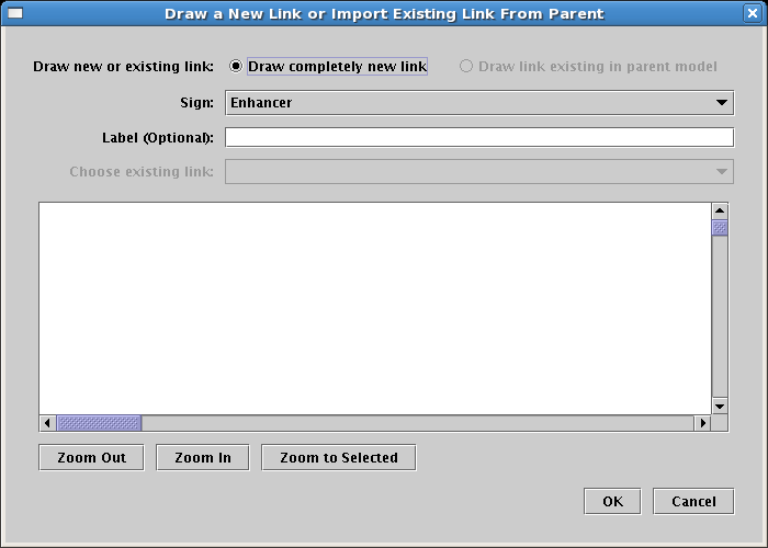
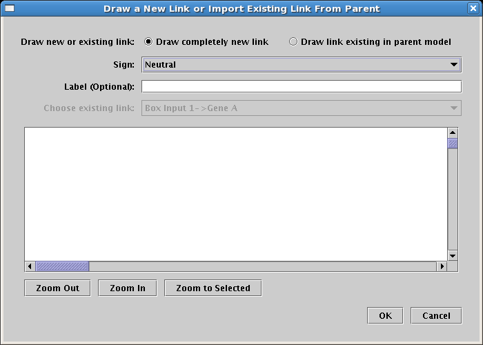
The dialog that appears again looks similar to the ones you have seen before, and provides you with the option of either creating a completely new link, or referencing an existing link that is already present in the parent model. Again, since the parent model has no links, the option is currently limited to creating a new link. The Sign selection will determine the type of arrowhead on the link; for this link, select a Sign of Enhancer. Adding a link label is optional, so just leave it blank, and click OK:
When you are placing a link, bubbles appear at the places where you can start and end the link. Just as with placing nodes, you can click on the Stop Sign button or hit the Esc key to cancel the operation. You will draw links by clicking the mouse to: 1) start the link, 2) add corner points, and 3) end the link. If you try to drag the mouse, BioTapestry will ask you to just use clicks. There are some restrictions on where you can start and end links. For example, you can't end a link on the same pad that a link is starting from, and on some nodes (like genes) you can only start links from certain pads and end links on other pads. If you pick an incorrect pad, BioTapestry will display an error cursor.
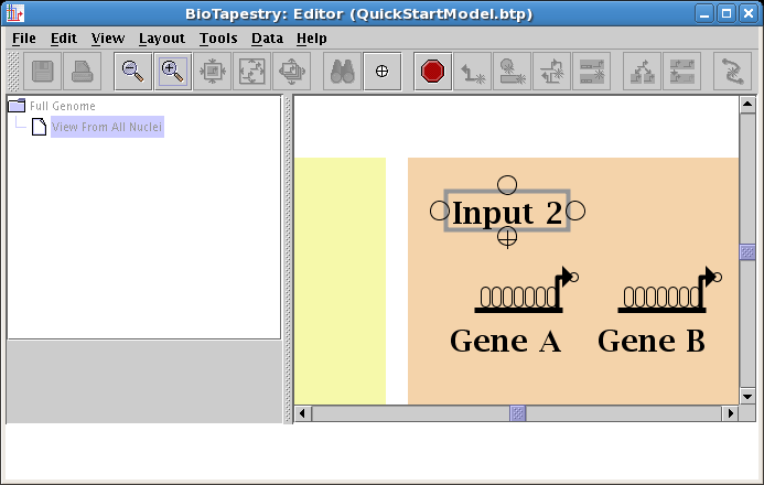
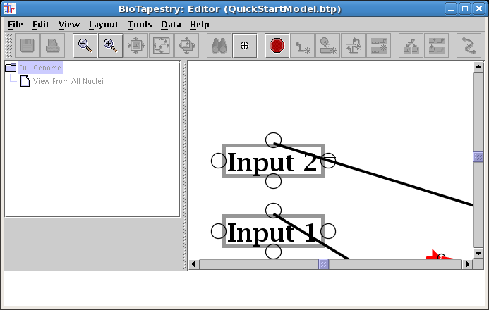
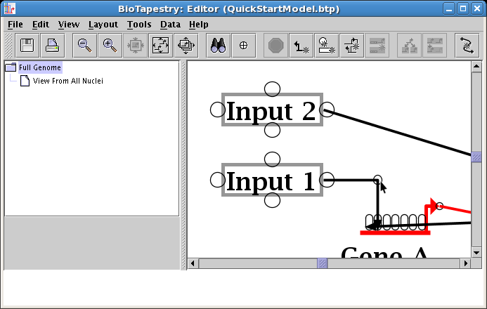
We will first draw a link in Region B from the bottom of Input 2 directly down to Gene A. (Note: you may want to zoom in now to view just the area detailed below.) Start by placing the crosshair cursor over the start bubble, and click the mouse:
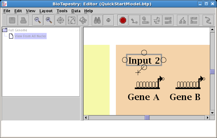
After starting the link, a thin black line follows the cursor around to show the link path:
Move the cursor over the target bubble:
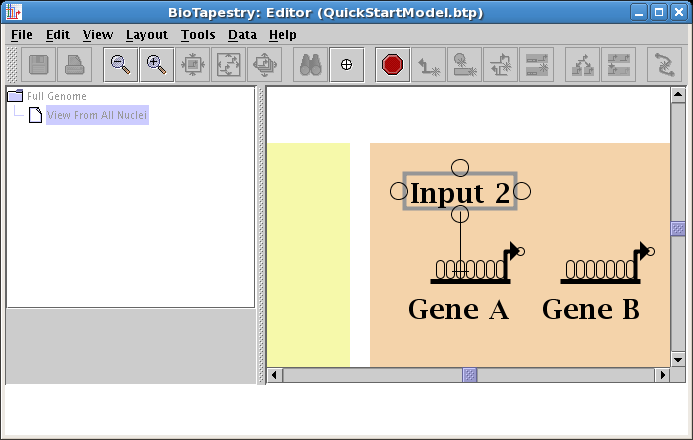
And click to finish the link. The placement is complete, and the link is now drawn in:
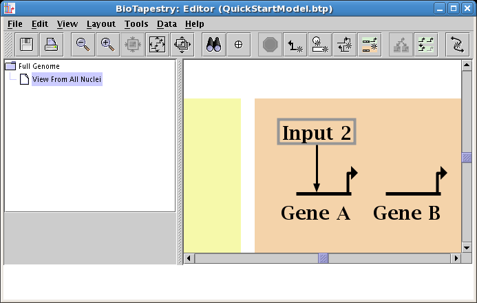
Create a second link, this time in Region A, from the right side of Input 1 to Gene A. Start as before, but this time click the mouse as the link is being drawn to create a corner point:

Next place the crosshair cursor over the target pad as shown and click to finish the link:
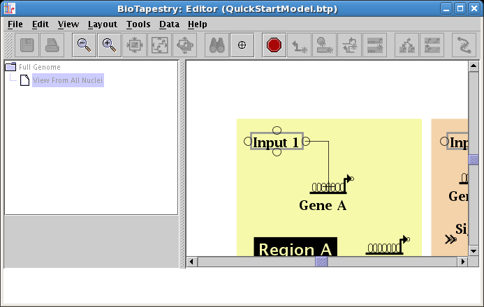
You are done:
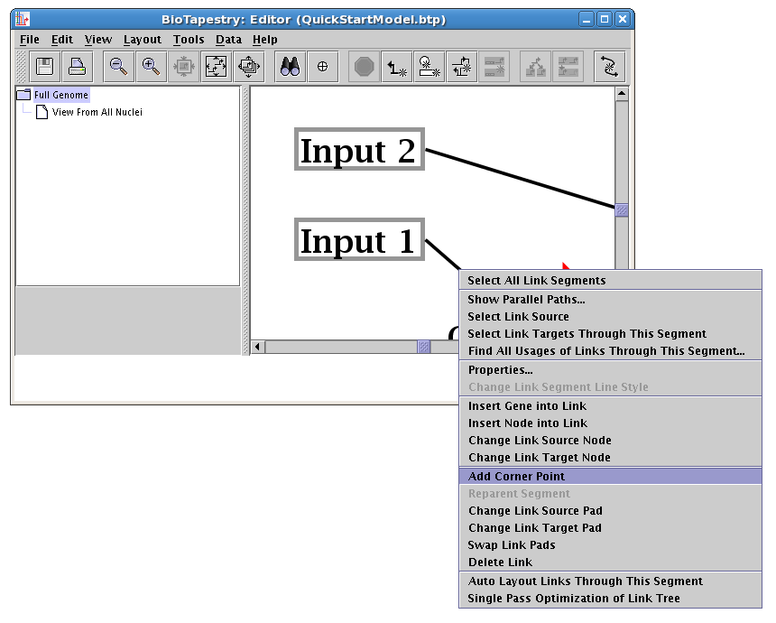
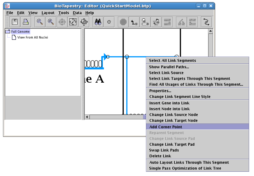
The essential thing to know about drawing the "circuit-trace" style of links in BioTapestry is that each node has at most one outbound "tree" of links. Once a link has been drawn from a node, all other links from that node must be started from somewhere on the existing link. Additional links originate from corner points, so if you don't have any bends in your existing link, or if the bends are not where you need them, you will need to add corner points. You are now going to go back over to Region B and draw the link from Input 2 to Gene B. If you recall, there were no corner points created when this link was drawn, so first right-click on the existing link from Input 2, and select Add Corner Point from the menu (again, note to Mac users: if you're using a one-button mouse, press the Control key while clicking the mouse to get the popup menu):
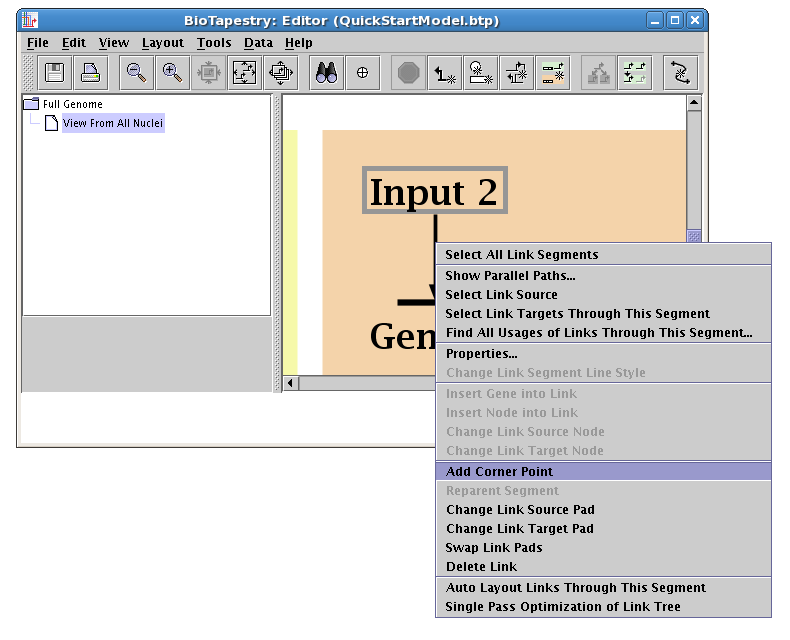
The corner point was added, but you probably cannot see it. During many link drawing and editing operations, the corner points are toggled on during the operation, but to see the corner points at other times, you can toggle the Toggle Link Pads button on the toolbar:

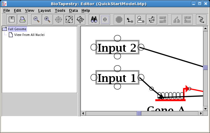
The places where you can draw links from and to are shown as bubbles. Begin as before: click on the Add Link... button on the toolbar, choose Draw completely new link, set the Sign of Enhancer, and click OK. But now make the first click on the newly added corner point:
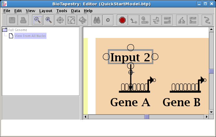
As you draw, add a corner point to create a bend, and then finish the link by clicking on a target pad on Gene B:
The next link will be from Input 2 to Gene C. Proceed as before, but since this will be a repressive link, select a Sign of Repressor on the link creation dialog:

And draw the link. Note how the repressor link has a foot instead of an arrowhead:
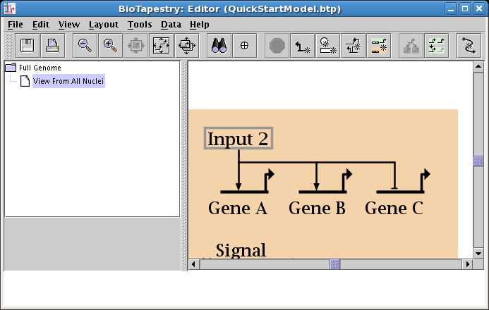
Keep drawing links. For the link from Gene C to the Signal node, the best presentation comes from assigning the link a Sign of Neutral, which draws the link without any arrowhead, so you get a cleaner looking signal node:
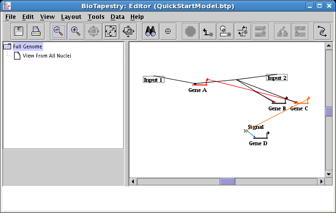
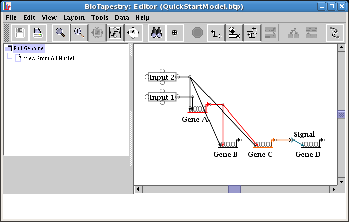
Continue adding all the rest of the links until the model appears as below. Colors are assigned automatically to genes and some other node types as soon as you draw a link from them, so the colors of your model may be different depending on the order in which you draw your links.
Note that none of the links you drew were copies of the same link in the top-level model, so they were all created using the Draw completely new link option. When you choose to create a link using the Draw link existing in parent model option, the program guides the drawing progress by selectively highlighting the available source and target nodes you can use which are consistent with the specified link you are trying to draw.
Once the network is drawn, you frequently want to change properties of some of the genes, nodes, or links, so this tutorial section will show how to modify some of these properties now.
Though the software does not currently do this automatically, the cleanest presentation would use the same color for a given gene present in multiple regions. So we want to change the color of Gene A in Region B to match the color in Region A, which (in this case) happens to be Sky Blue. To change gene properties, right-click on the gene, and select Properties... from the menu:
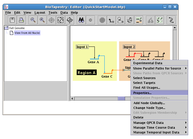
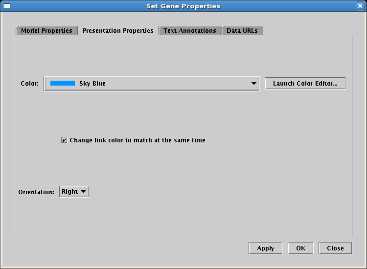
There are several tabs in the dialog that appears. So-called Model Properties (like the name, or the cis-regulatory module specification) appear on the first tab. For gene color, select the tab named Presentation Properties, and set the color to match the other copy of Gene A (in this example, it is Sky Blue). Note that the default is that the link color will be changed to match at the same time. Click OK, and the gene and outbound link colors will be changed:
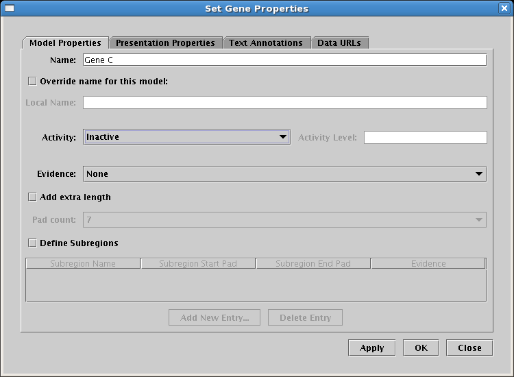
The next thing to do is to set the copy of Gene C over in Region B so that it appears greyed out, i.e. it is inactive. In many model hierarchies, this second-level model is used to show all the genes and links that are active during some time span, so nodes are links are typically fully colored in at this level, and time-dependent active and inactive components are depicted in the next model level down. However, because Input 2 is repressing Gene C in Region B for the entire time under study, we prefer to show that instance of Gene C as always inactive. While you could do this by changing the gene color to grey, the preferred approach is to specify the gene activity level as inactive; this is a property of the model, not of the specific layout of the model. (In a similar fashion, links can also be set as inactive at this level, via the Link Properties dialog you can access by right-clicking on a link.) Access the properties dialog by right-clicking on Gene C and selecting Properties... from the menu. Then, on the Model Properties tab, set Activity to Inactive, and click OK:
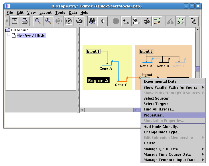
The last step to complete this model is to clean up the presentation of the Signal node. To do this, right-click on the node and select Properties...:
Select the Presentation Properties tab on the dialog. We want to hide the Signal node name, so check the Hide node name box. Also, we want to change the Color of the node to match the inbound link (the Second Color probably already matches the outbound link color). Here it is set to Pumpkin Orange, but the color you select may be different, depending on the order you used to draw links:
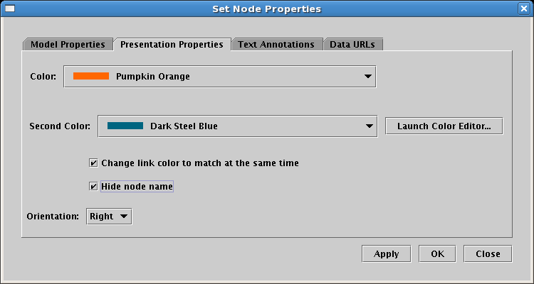
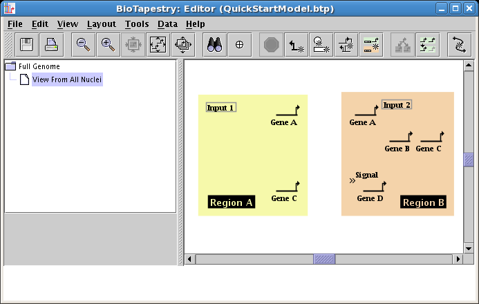
Click on OK, and your model is done; it should look like the network below. It's a good time to save your work!

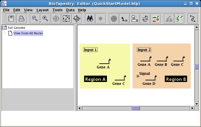
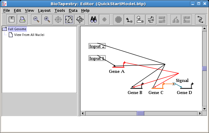
It's time to go and check the top-level Full Genome model that was automatically created as you drew your second-level model. In the navigation pane on the left, click on the Full Genome model to select it. Most likely, it is a real mess:
BioTapestry does not attempt an ongoing real-time effort to keep the top-level model layout in sync as you modify lower layouts. In this case, nodes and genes were dragged around after they were first drawn, but here they are still in their first-placed locations. Plus, the different gene locations meant that when links were first drawn, the simple rule of duplicating the link layout in the top-level model couldn't be applied, so BioTapestry didn't spend the time trying to come up with an alternative. But now that you are done building the lower network, you can sync things up.
As was mentioned at the start of the tutorial, there is a tool to help keep the top-level model layout in sync with other model layouts (see Layout->Propagate Layout to Full Genome Model...). It may not be obvious how to always do this automatically (i.e. if there are many second-level models with different layouts, and multiple regions in each model with unique layouts of different pieces of the top-level network, which do you want to use?) The tool helps you to specify and remember a strategy to use for this task.
But since this is a simple layout, and since this exercise will help to teach crucial link-editing techniques, we will now clean up this layout manually. The first thing to do is to drag nodes around to the positions shown below (don't bother with the links for now). Note that this network is going to be organized differently from the second-level model!
NOTE: It's likely that the link arrangement in your model is at least slightly different from that pictured below. If it turns out that you cannot exactly follow the editing steps we describe below due to the differences, you should still be able to perform roughly equal editing operations to what we describe.
You do not, as a rule, want to delete links and redraw them, since when you have submodels, the act of deleting a link removes them from all the submodels! Instead, always retain your links, but just edit the layout of a link. To begin, a very common operation is to change where a link leaves and lands on a node. In this case, we now want the link out of Input 2 to start on the right side of the box. Right-click on the link and select Change Link Source Pad:
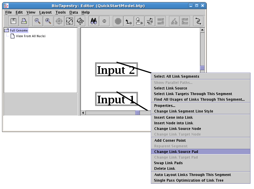
The cursor changes to a crosshair. You now just click on the new source pad:
The link start is now switched:
Repeat this step for the link out of Input 1, again having the link start on the right side of the box:

Next, we want to make the link from Input 1 to Gene A orthogonal. To do this, you will first need to add a corner point to the link. Right-click somewhere in the middle of the link and select Add Corner Point:
As before, you might need to toggle the Toggle Link Pads button on the toolbar to be able to see the new corner point:
Corner points can be dragged just like genes and nodes. Place your mouse cursor over the corner point and drag it over until the links are orthogonal:
Now do the same thing with the other corner points that are already in the link trees, which is the first step towards making all the links orthogonal. After you are done, the network will look something like this:
Then add new corner points where needed to make most of the other links orthogonal (see below). Note that in the resulting layout, we are left with a diagonal link from Input 2 into Gene B. The crucial point to note right now is that you do not want to make this link orthogonal by adding a corner point to the diagonal segment and then dragging the corner point over on top of the existing link from Input 2 to Gene C. The result will look almost correct, but you will end up with a link tree that behaves unexpectedly when you click on the overlapping segments, acts poorly when applying automatic layouts, and displays similar undesirable side-effects. To deal with this situation, you will want to edit the tree to "reparent" the diagonal link:
Reparenting a link segment is the single most important skill to know for manually editing links! As nodes are moved around, you are going to frequently want to rearrange how a link tree is laid out, changing where some portions of the link tree attach to other portions. There are tools to help you do this (e.g. you can right-click on a link segment and select Auto Layout Links Through This Segment), but the best final layout is often created or tweaked manually. So to change where a link segment attaches in the tree, you will right-click on the segment and use Reparent Segment.
In our example, you will first need to create a new corner point in the segment just above the target pad on Gene B:
Then right-click on the diagonal segment you want to relocate, and select Reparent Segment:
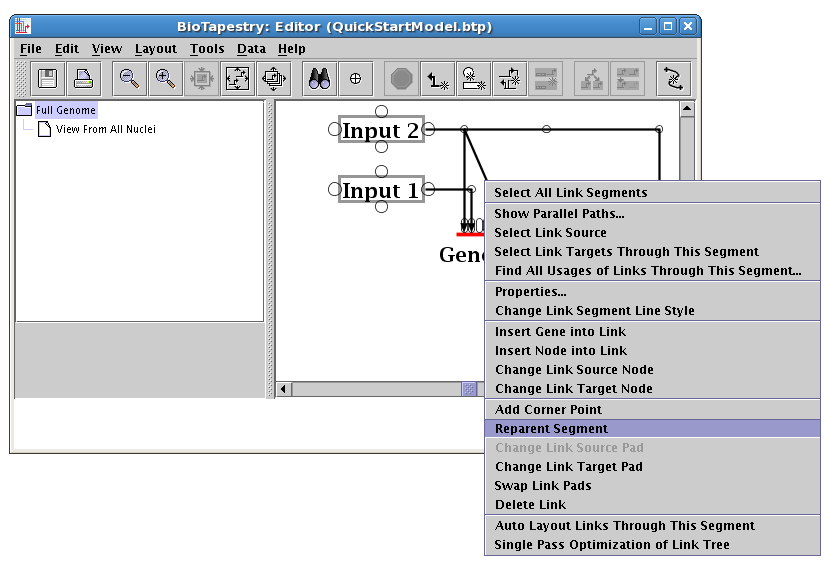
Your cursor will change to a crosshair. You will place the crosshair over the new corner point:
When you click the mouse, the segment will change where it attaches to the link tree. Drag the corner point as needed to make the link orthogonal (see below).
It's good to get familiar with doing these rearrangements; sometimes you need to think geometrically to plan how to rearrange a link tree, and you don't want to get in the habit of just overlaying and stacking multiple link segments on top of each other to make things "look" right while creating confusing link tree structures. Keep in mind that sometimes when you click on a corner point to finish reparenting a segment, the program won't let you; it may be that you have tried to reorganize the link tree in a way that would orphan a chunk of the tree, completely detaching it from the link's source node. The software detects these cases and guarantees the link tree is kept consistent.
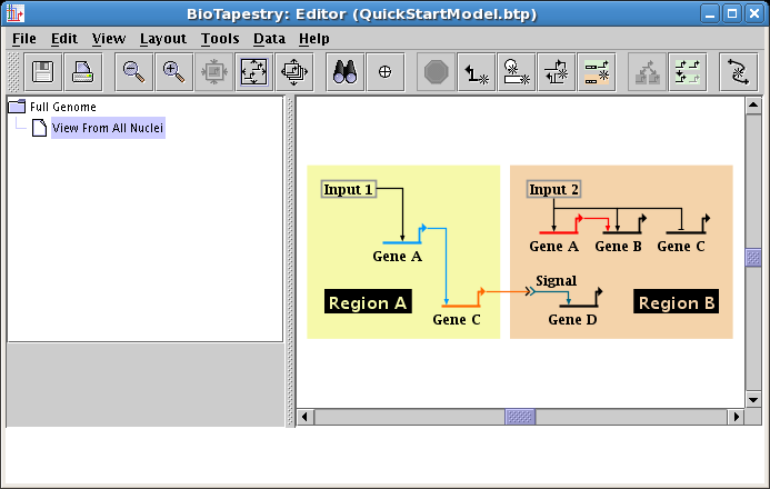
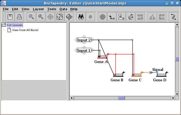
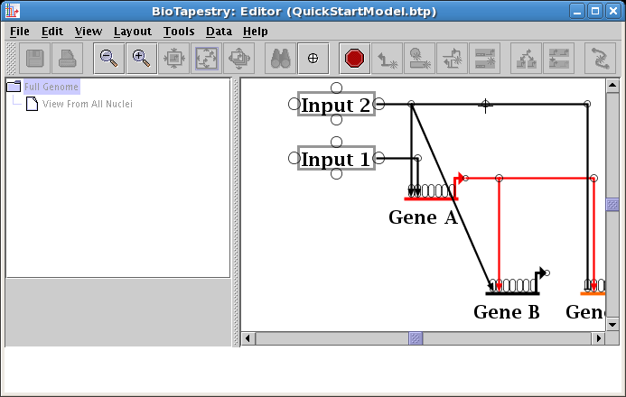
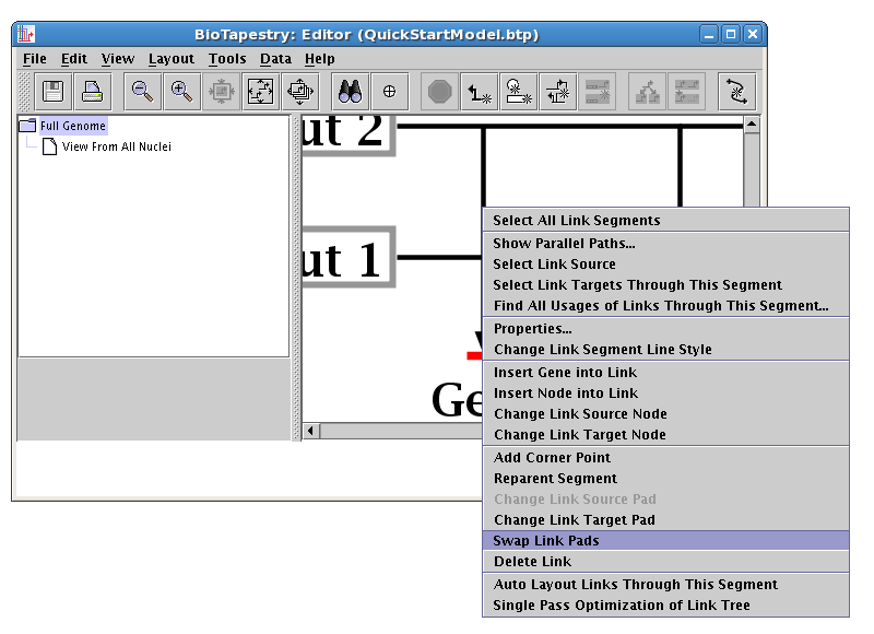
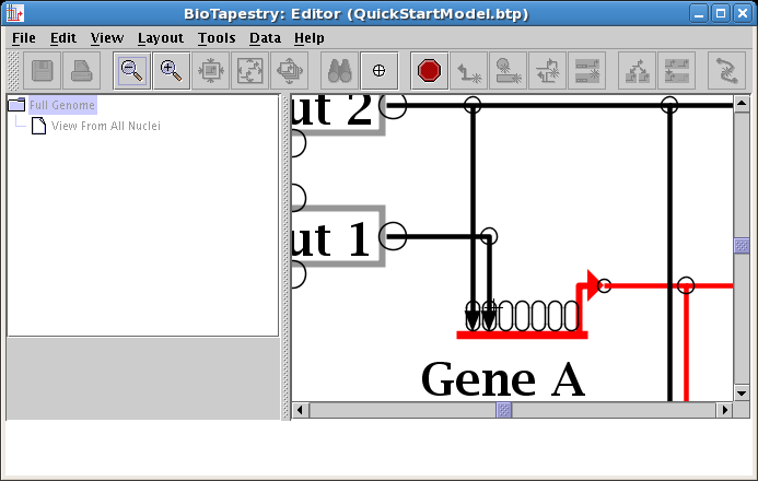
A few steps ago, you learned how to change the source pad where a link originates from. It's not a surprise that you can do the same thing to where a link lands (the target pad). But since you often have multiple inbound links into a gene or node, you can speed up things by swapping the landing pads of two nodes at once. Our example network (see below) illustrates one case where you want to do this; the two different inputs into Gene A cross over each other (with the same color). A cleaner layout will eliminate the link crossing by swapping the two landing pads. Note that sometimes the ordering of the links inbound to a gene is important (as it would be if you were trying to match the known ordering of cis-regulatory binding sites). But if this is not the case, the layout is improved by picking an input arrangement with the cleanest layout.
To do this cleanup, right-click on one of the links (here we choose the link from Input 2), and select Swap Link Pads from the menu:
With the crosshair cursor, lick on the landing pad where you want the link to go (in this case, the pad where the link from Input 1 lands:
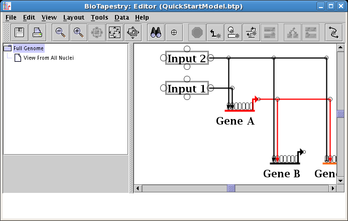
This causes the two links to swap landing locations. Now drag the corner points to make things orthogonal. It is frequently best to first drag the corner point closest to the target, since moving the longer link first may make it hard to drag the shorter link's corner out from under it. In this case, do the link from Input 1 first:
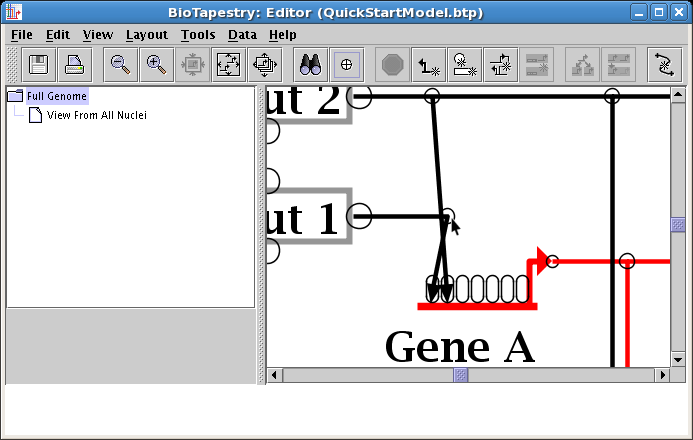
Once you have dragged the corner points, you are done:

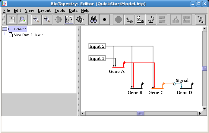
In our example, the same cleanup should be performed on the two inputs into Gene C, which also have an unnecessary crossing. Do another target pad swap on those inputs, and your resulting layout should look like this:

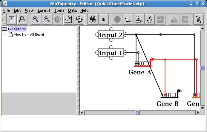
Next we will show how to move several segments of a link tree all at once. To begin, drag the Input 2 node down a little bit, leaving the diagonal outbound link alone:

To get this link tree square again, you could drag segments or corner points around one at a time. Instead, click on one of the two horizontal segments to select it, then Shift-click to select the second segment while keeping the first selection. The Shift-click (hold down the Shift key while clicking the mouse) is one way to keep adding network elements to your selection set. Alternately, you can drag a rubber-band box around the two segments by pressing down the mouse button over an unoccupied part of the workspace, dragging the mouse to box in the two segments, and releasing the mouse. Either way, you should have just the two links selected:

Now drag one of the selected segments down to square up the link; the other one will follow (see below). When you are done, click on an empty space in the network, or select Edit->Select None from the main menu, and the selections will be cleared.
At this point, you will want to clean up the colors and labels, just like you did before for the second-level model (see Editing Node Properties above). Since colors and label-hiding are set by the layout, and layouts between the models are independent, these changes need to be done for this model too. Change the color of Gene A to match the color used in the second-level model (it was Sky Blue), and change the Signal node to hide the label and set the colors (it was Pumpkin Orange and Dark Steel Blue). Your top-level mode is done (save your work!):
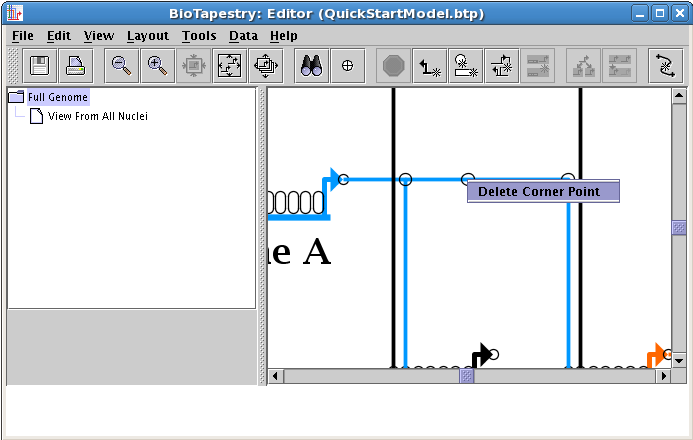
One editing task which was not covered so far is how to delete corner points. Corner points that are used for the intersection of two or more links cannot be deleted, as they are required to maintain the tree structure. However, corner points that just form corners, or which are sitting on a straight segment run, can be deleted. While unused corner points are generally innocuous, cleaning them up may make link drags go more smoothly and eliminate surprises when right-clicking on a straight link run.
Since the finished model probably doesn't have an unused corner point, we will add one. Add a corner point to a segment:
Be sure to toggle the links pad on to be able to see the point:

Right-clicking on the corner point brings up the only option: Delete Corner Point. Do this now. If a corner point is supporting an intersection, this option will not be enabled.
The final task at this point is to line up the layout of the top-level model with the layout of the second-level model. As nodes get moved around, the two layouts can get shifted away from each other. In this example, if you center the top-level network (click the Zoom as Needed to Show Current Model button on the toolbar) and then select the View From All Nuclei model, the latter is offset in the view:
There are tools available to line up the networks. From the main menu, select Layout->Layout Centering and Alignment->Align Centers of All Model Layouts...:
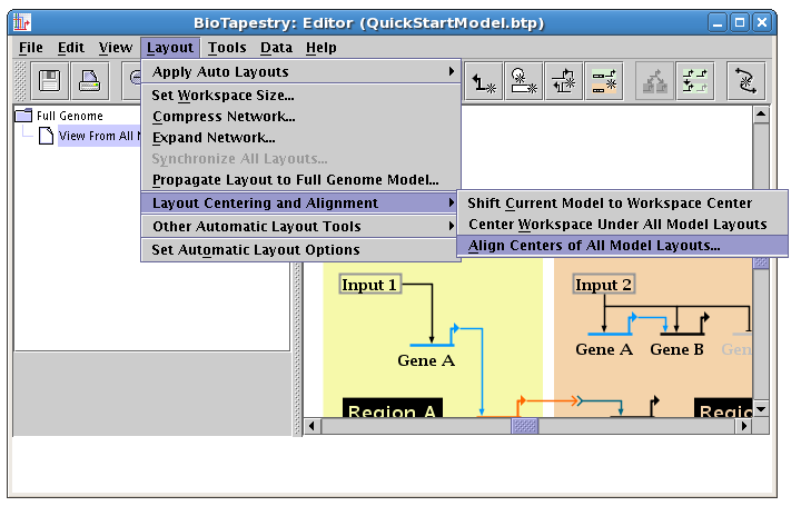
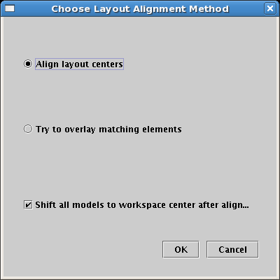
In the dialog box that appears, select Align layout centers, and check the box to Shift all models to workspace center after alignment. Click OK:
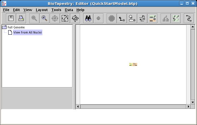
You will see the current model, zoomed out all the way to show that it has been centered in the workspace:
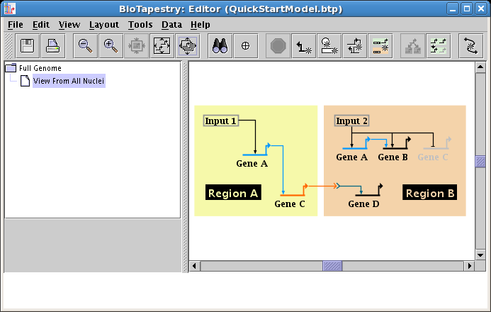
When you then click the Zoom As Needed to Bound All Models in Hierarchy button on the toolbar (the rightmost zoom button) you will center the current model (see below). Selecting the Full Genome model will show it is centered too.
To complete the tutorial, we will create two new models at the lowest level of the model hierarchy. Each of these models will show the parts of the network that are active at an early stage of the time period of interest. Right-click on the View From All Nuclei model in the navigation pane, and select Create Submodel:
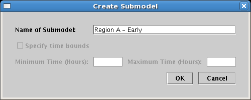
Set the Name of Submodel in the dialog to Region A - Early and click OK:
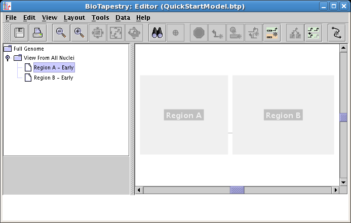
Do this again, but name the second model Region B - Early. When you are done, make sure you have created these two models as child models below the View From All Nuclei model, and not as child models of the Full Genome model! Click on the Region A - Early model in the tree to select it, as we will populate this model first. You should see this:
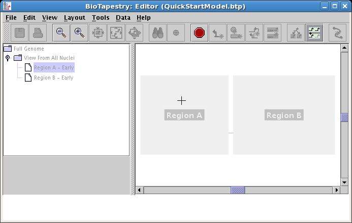
At this level in the model hierarchy (and below), the models share the network layout of the second-level parent model. As of Version 3, you can draw things into this model directly if you wish, but at this point it is usually simplest to just click on which ghosted elements in the parent you wish to include; any element you do not included remains ghosted. To begin populating this model, click on the Choose Subset of Parent toolbar button:

You will now remain in this selection mode until you hit the Esc key, click on the Stop Sign button, or toggle off the Choose Subset of Parent button. To begin, place the crosshair cursor over the ghosted Region A and click:
Region A will then appear colored. Then click on all the nodes: Input 1, Gene A, and Gene C, as well as the links between them. Exit from the choose mode using one of the methods listed above (e.g. click on the Stop Sign). This produces the following model:
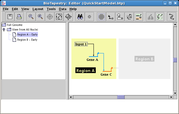
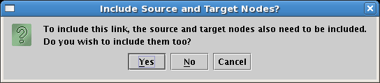
It is not possible to include just the link between two nodes without also including the nodes themselves. In fact, if you click on the link before including the endpoints, you are presented with the following dialog, requiring you to make the choice:
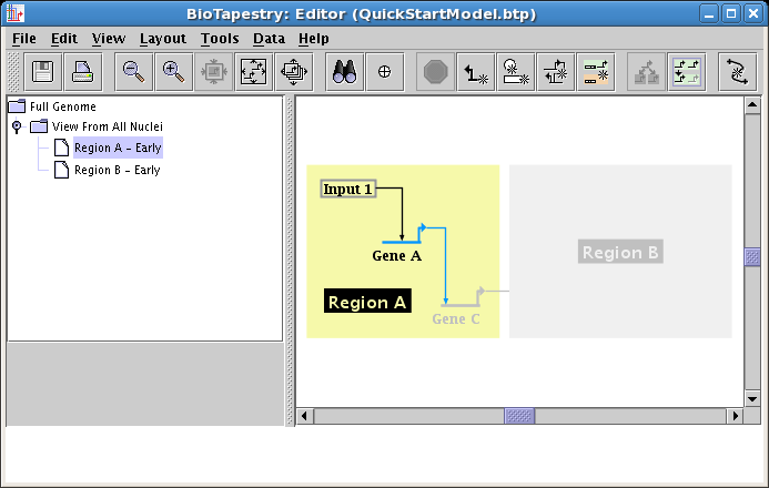
The typical usage of these submodels is to show just the fraction of links and nodes that are active in some set of conditions, while showing the inactive parts as ghosted. Whatever is not included from the parent appears in this ghosted state automatically. However, you may want to show a target gene as not yet expressing, even though the link into it is active. As we just saw, you cannot include just the link without also including the target. In these cases, you need to include the target, and then set its activity level to inactive. We covered this topic while building the second-level model. So after including Gene C, set it to Inactive, and you will then have the final version of this model, showing the early state of Region A:
The Region B - Early model is built in the same fashion. After choosing the model and clicking on the Choose Subset of Parent toolbar button, click on Region B, then click on the link out of Input 2, and answer Yes when asked if you want to include the targets.
This is a good time to discuss the concept of which links are "passing through a segment" of the link tree. Looking at the links out of Input 2, there are a total of three: one each to Gene A, Gene B, and Gene C. Looking at the link tree, you can think of all three links "passing though" the link segment immediately below the Input 2 box node, before the first branch. So if you click on that first segment, you are telling the program you want all three links to be pulled down from the parent. If you instead click on one of the link segments immediately above the landing pad on one of the target genes, which is not shared by any other link, you are telling the program you just want that one single link. The link segments between these two extremes handle some subset of all the links out of a source, which you can reason about by looking at the tree. This sort of link-bundling logic applies to several link operations, e.g. when you right-click on a link segment and select Select Link Targets Through This Segment.
Once you have pulled down the links, the model should appear as below. Note how Gene C is already tagged as Inactive, since it is inactive in the parent model, so it appears grey even though it has been included. In fact, a node at this level cannot be made active if the parent model's node is inactive; the submodel is guaranteed to be a consistent subset of the parent model, including allowed expression levels.
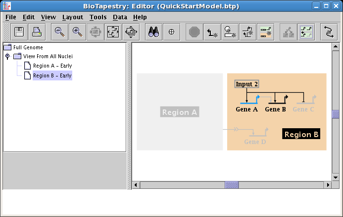
Finally, since Gene B is not yet expressing at this early stage, set it as Inactive using the Gene Properties dialog, as we have shown above. That will give us the finished model:
This QuickStart Tutorial was designed to walk you through the basic steps involved in building a multi-level genetic regulatory network model hierarchy in BioTapestry using the drawing features. The lower level models that you created were static submodels, i.e. they represent a single snapshot in time, and you create them by manually specifying what network elements to include. There are other tutorials available on the BioTapestry site that step you through the process of creating dynamic data-driven models, building models using interactions lists and spreadsheet inputs, and other advanced topics, If there are any other questions about using the program that are not covered by these tutorials, the online FAQ is a good source for answers. There is also a Google group called BioTapestry-users where you can ask questions and get more information.