|
|
|
|
|
|
|
|
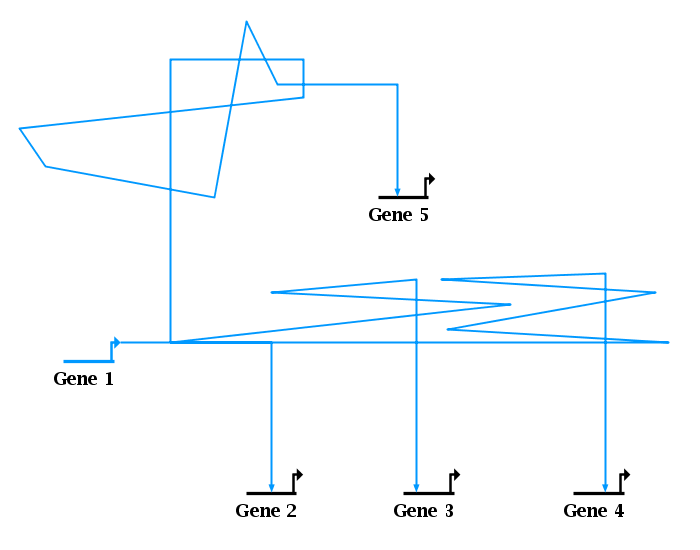
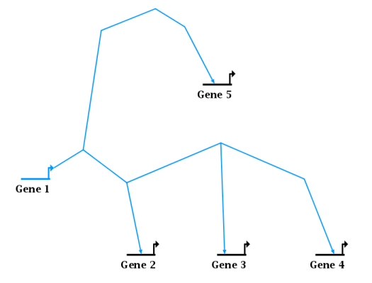
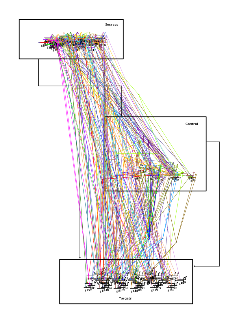
Just because a link tree looks good doesn't mean that it is constructed well, and the new link geometry repair feature makes it easy to quickly fix problems with link trees. To illustrate this feature, consider the link geometry in the picture below, which needs significant clean-up:
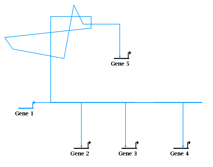
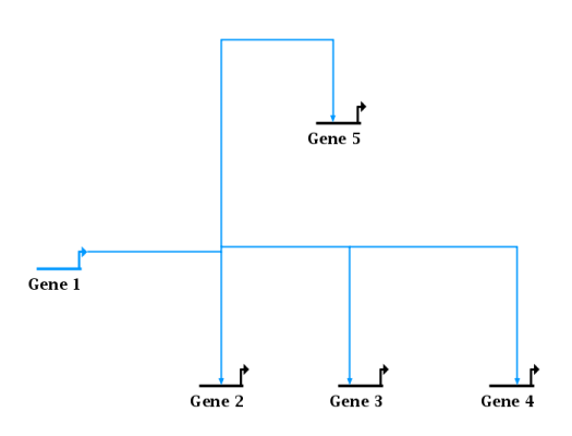
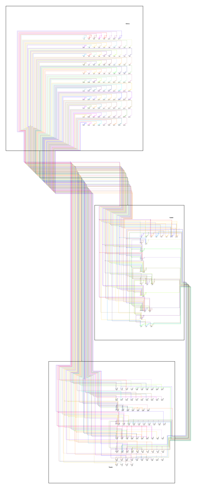
It may seem that the easiest way to clean up the mess in the lower half of the network is to just drag the link corners down so that all the overlapping segments lie on the horizontal line, giving the network shown in the picture below. The only difference between these two images is that all the lower zig-zags are hidden because they are now overlapping. But this is not the best way to leave things! While it may superficially look OK (except for the overhang on the right end and some subtle irregularities in the link thickness), it can lead to unexpected problems. For example, right-clicking on a segment to interrogate what links are passing through it, or what targets are downstream, can give misleading results when multiple segments overlap. Also, simple autolayout operations can give poor, unexpected results when link segments are overlapping.
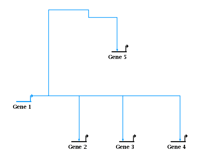
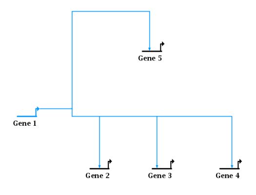
Version 6 now includes a feature that can easily clean up these problems. To fix a single link tree, right-click on any segment in the tree and select Link Layout Operations->Clean Up Overlapping Link Tree Geometry from the menu. To fix all link trees in the layout, select Layout->Clean Up All Overlapping Link Tree Geometry from the main menu. Not only will this clean up the invisibly overlapping segments, but it will also handle cases as shown at the top, where extraneous link segment loops are thrown away:
This feature promises to make link construction and modification much faster and easier, since all one needs to do is to make a link tree look plausible, and then apply the repair step to make the tree well-formed.
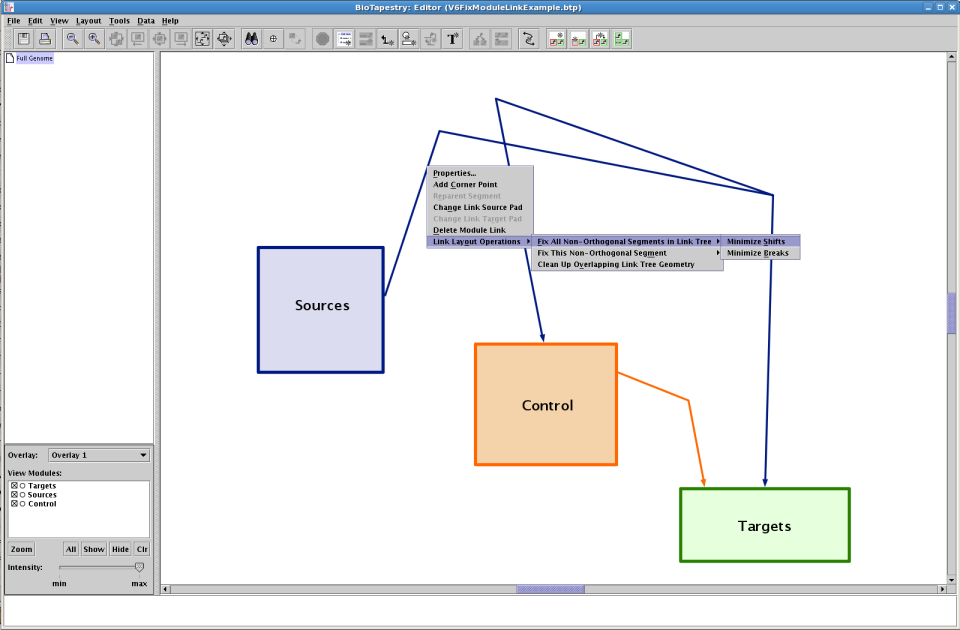
BioTapestry network layouts are intended to display neat, orthogonal link trees. There has long been built-in support to help draw orthogonal links by holding down the Shift key while moving and clicking the mouse. But as node and links get dragged and edited, the orthogonality is usually lost, and trying to fix it by doing a complete auto-layout of the link tree typically produces an entirely different, and unintended, routing strategy. Instead, you want the system to be able to gently tweak the approximate existing routing to just straighten out the links, thereby avoiding any huge changes. Version 6 introduces a feature to do this tweaking for most cases. For example, consider the following layout that is basically what we want, but with crooked links:
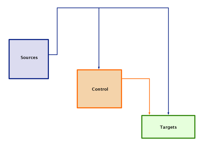
To clean up diagonal links for a single tree like the above, right-click on any segment in the tree and go to either Link Layout Operations->Fix All Non-Orthogonal Segments in Link Tree or (when the clicked-on segment is itself crooked) Link Layout Operations->Fix This Non-Orthogonal Segment. Each of these options leads to a final menu choice, where you can select to either Minimize Shifts or Minimize Breaks. This choice specifies the preferred strategy for clean up. The system will either tend to keep existing corners in place and create new corners (mimimize shifts) or move existing corners to avoid creating new ones (minimize breaks). For example, this shows the strategy to minimize breaks:
While this example shows the result of minimizing shifts:
Note that you can apply this operation to an entire layout instead of just a single link tree, by choosing Layout->Fix All Non-0rthogonal Segments from the main menu, and finish by selecting one of the same two strategy options described above.
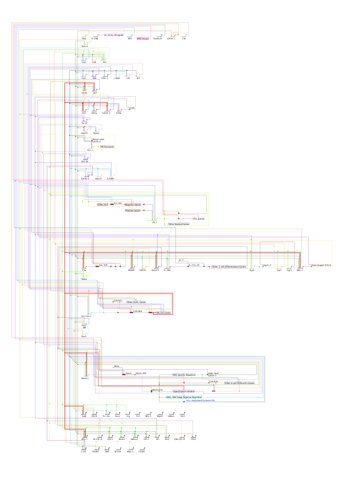
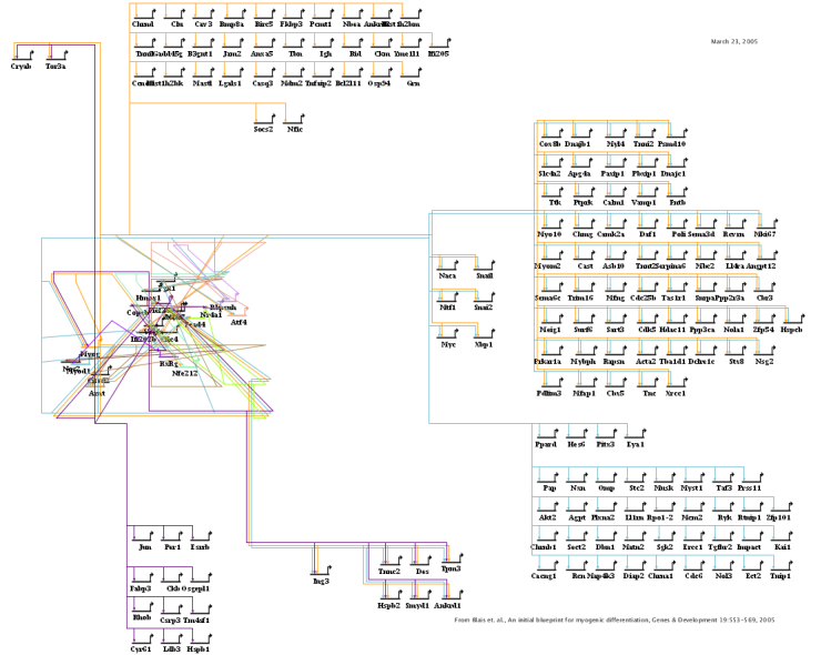
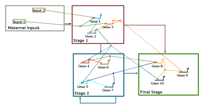
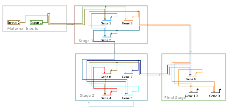
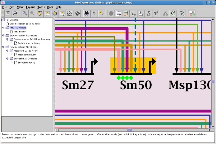
Version 6 introduces a new automatic layout format, the Stacked Strategy. This new strategy augments the previously offered Alternating, Diagonal, and Bipartite strategies, and forms the basis of the other new layout features introduced in Version 6. The stacked strategy continues to use the established technique of gene-centric organization, where non-gene nodes are grouped near their associated source or target genes. (Note that this means that intercellular signal nodes are not treated specially and placed on region boundaries; that is a planned future enhancement.) As the figure below illustrates, the approach creates a vertical stack of gene rows, with inputs and output links routed above each row, and inter-row links routed down the left side as a unified bundle. (This example is a reorganized version of the T-cell network available from here):
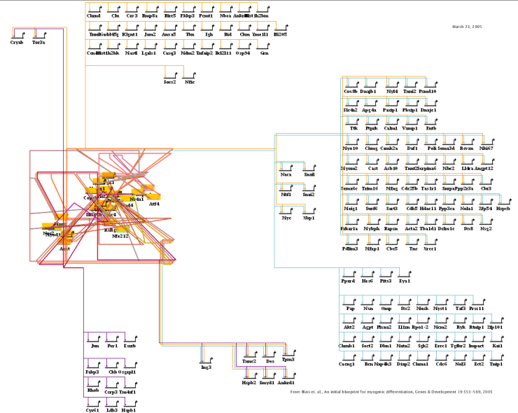
Before Version 6, the auto-layout strategies could only be applied to the entire network at the top (Full Genome) model level. Now (still only for the Full Genome model), the user can select a subset of the network nodes and just have that part laid out, leaving the remainder of the layout unaffected. With this release, the stacked strategy (described above) is supported, and the user is responsible for arranging the network as needed to create enough space for the auto-layout to succeed. For example, in the following network, we want to layout only a set of genes, while not changing anything else:
The first step is to select the nodes that need to be reorganized. This multiple selection can be easily done using a rubber-band box:
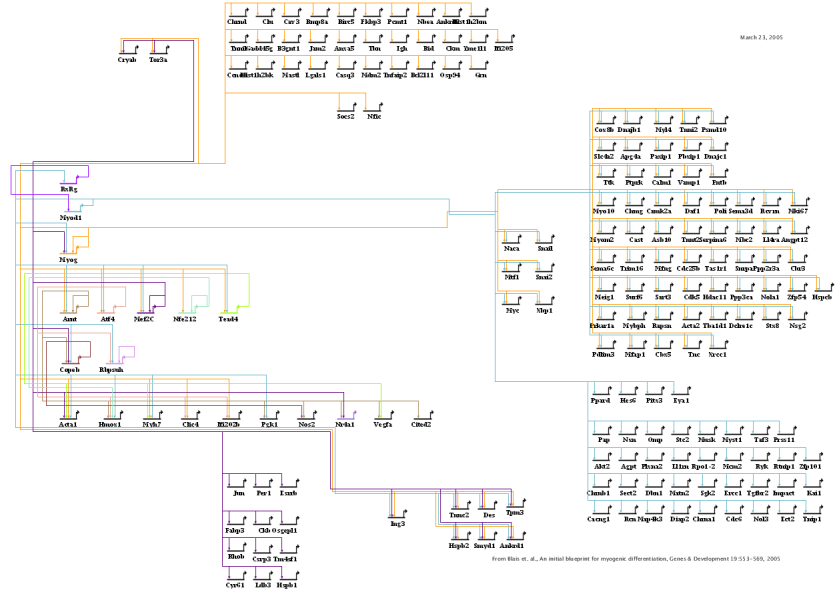
Then, from the main menu, select Layout->Apply Auto Layouts->Selected Only, set any desired options in the popup dialog, and click OK. Only the selected nodes will be reorganized:
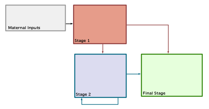
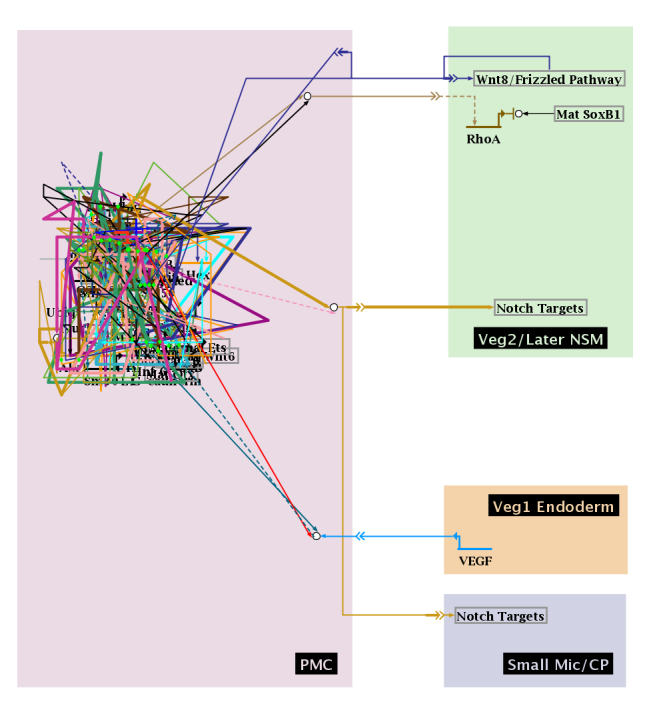
Network overlays with network modules were introduced in Version 4 (see Version 4 Release Notes). This feature allows the user to create a high-level abstract process diagram that describes the overall architecture of a network:
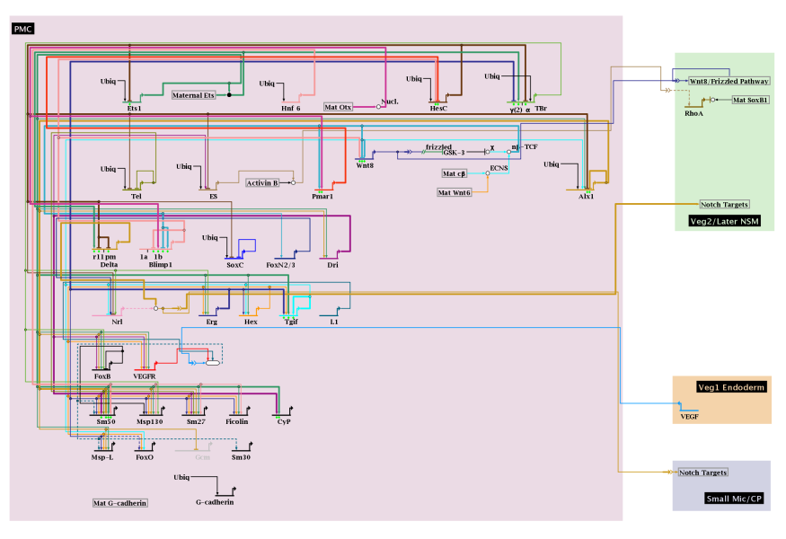
Version 6 now supports the automatic layout of a network that conforms to an overlaid process diagram. The user simply needs to assign each node to the appropriate module, as shown in the figure below. Also, the network overlay needs to conform to certain guidelines:
Once the above requirements are met, select Layout->Apply Auto Layouts->Per Current Overlay, set desired parameters in the dialog box, and hit OK. The nodes inside each module are laid out with the stacked template, and inter-module links are arranged to follow the paths of the network module links:
The overlay-based layout tool is designed to expand the process diagram as needed to accomodate all the nodes and links. For example, consider this starting point, where a large number of nodes and links have been crowded into three small modules:
After applying the overlay layout, the geometry has been expanded as needed:
In previous versions, two automatic layout strategies were listed: General and Bipartite. In Version 6, the strategies have been reorganized. The previously named General strategy had separate parameter settings that made it behave quite differently, so it has now been split into two: Diagonal and Alternating. These now appear alongside all the newly added features as shown below:
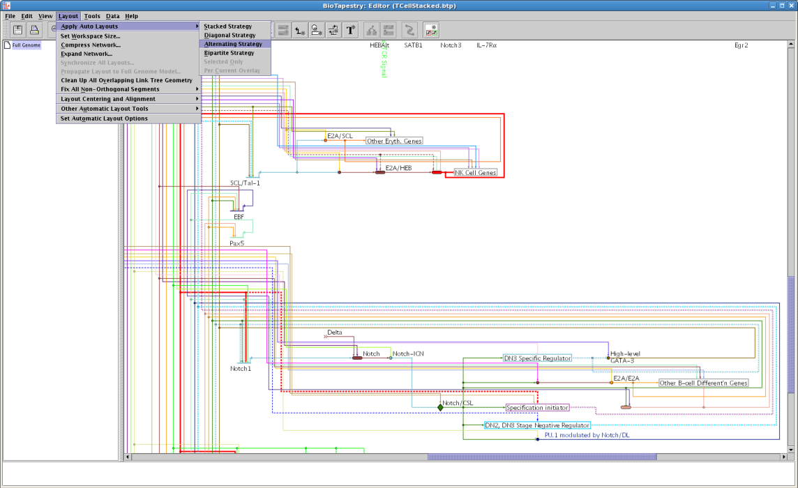
Layout options below the top-level Full Genome model were previously limited to synchronizing with the top-level model, expanding, or compressing. Now, each region can individually be laid out automatically using the stacked strategy. In the following example, we want to apply automatic layout to the PMC region:
With the mouse, right-click in an unoccupied part of the PMC region and select Layout Region... from the popup menu. Set the desired parameters in the dialog box, and hit OK. The region will be laid out, after having been expanded as needed to accomodate the new size:
The new features that have been added for cleaning up and orthogonalizing links are also available for network module links. This is useful, since network module links need to be orthogonal and well-formed before they can be used as part of an overlay driven layout. For example, we want to clean up the network module links in this overlay:
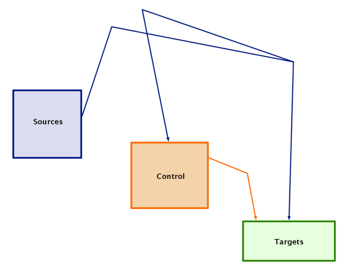
With the mouse, right-click on a network module link segment region and make the appropriate selection from the popup menu; this menu is similar to the one offered for regular links:
After both link trees have be cleaned up, the overlay should look like this:
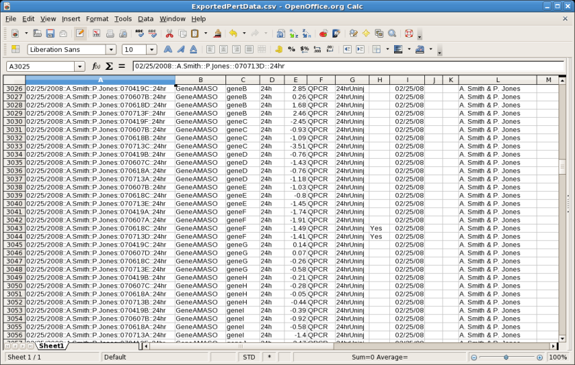
Version 5 (see Version 5 Release Notes) introduced an extensive overhaul of the system for storing and displaying perturbation data. A new export option has now been introduced that allow the user to write out all the perturbation data to a comma-separated value (CSV) file. From the main menu, select File->Export->Export Perturbation Data to CSV..., and save the file. It can then be imported into a spreadsheet program:
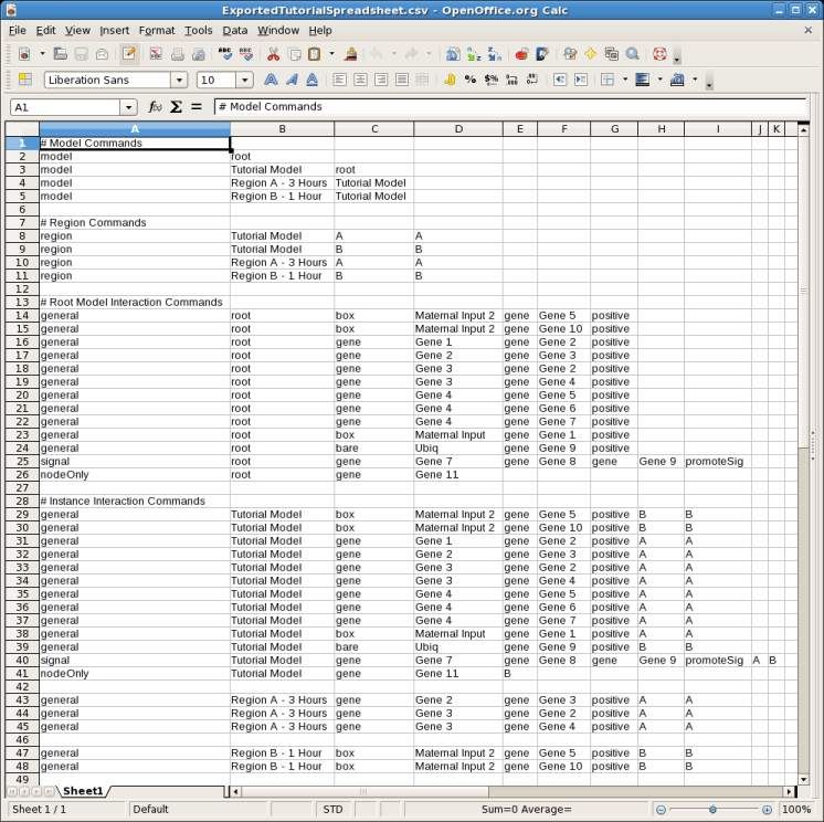
BioTapestry has long supported the ability to build a network using interaction tables (see the tutorial Building Networks from Interaction Tables) and from a CSV file import (see the tutorial Building Networks from Comma-Separated Value Files). Both these methods create an internal list of build instructions. Version 6 introduces the ability to write out these instructions to a CSV file using the same format used for importing. From the main menu, select File->Export->Export Build Instructions to CSV..., and save the file. For example, here is the export of the sample CSV file used in the CSV file import tutorial mentioned above:
Searching for node sources and targets has previously been limited to only direct (i.e. one-hop) searches. But this meant that discovering paths through non-gene nodes (e.g. bubbles, signals, slashes) to reach terminal genes would require multiple selection steps. Version 6 now provides the ability to pass through intermediate non-gene nodes to reveal the eventual gene sources or targets. This feature is available from the popup menu when you right-click on a node. As shown below, the options to Select Sources or Select Targets now lead to a further choice of simply selecting direct connections or using the pass-through method. Note as well that the user now has the option of choosing whether to include the relevant links in the selection, as well as the ability to include the query node as well, though these two options are only applicable to the direct connections search method. For pass-through searches, all nodes in the paths (including the query node) are included, but links are omitted.
The pop-up menu below also illustrates another new feature related to search selections, which is the ability to keep appending selections through successive searches. Previously, each search cleared the existing selection set (this option is also now provided in the general search tool):
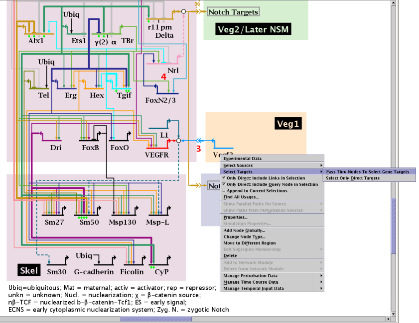
The picture below shows the result of a pass-through search for the gene targets of Vegf3. Note how both the gene targets, as well as the intermediate nodes in the path are selected:
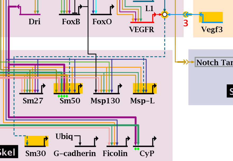
Previous versions of BioTapestry provided a toolbar button to zoom to bound the selected objects. This worked well when the selected objects were generally localized to a small area. But when, for example, the selections were the result of finding all targets of a gene in a very large network, this feature did not provide the necessary functionality. Thus, in Version 6, there are new buttons that allow the user to cycle through each object in the selected set, and zoom to the current object. There is also a button to clear all selections. Thus, the toolbar now has (in order, starting from left, referencing just the highlighted buttons):
So, given the set of Vegf3 target search results above, cycling through the selections allows the user to see each target up close:
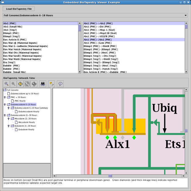
If you want to include the BioTapestry Viewer as a component of part of larger Java program that deals with gene regulatory
networks, Version 6 provides a new interface for doing this. An example of how to do this is shown in the class
org.systemsbiology.biotapestry.embedded.EmbeddedViewerPanelTestWrapper in the source code. The following
image shows a screen shot of this test wrapper. Note how the calling program is able to specify which model to show,
and which network elements to zoom to. It also is able to listen for model and selection changes, and query to find out
what models and elements are present:
Version 6 tries to do a better job of handling mouse-click intersections of network elements. In particular:
Last updated: September 5, 2023
biotapestry at systemsbiology dot org